Abstract
The OpenScope Community Project consist of team-based open science on a large international scale. Every step of the scientific process is performed in a maximally transparent and inclusive fashion. Anyone around the globe can join and contribute to the project at any point in time. Contributions are preserved, kept public, and freely accesible. The initial project centers on predictive processing, a popular theory in systems neuroscience which assumes brain responses to mostly reflect deviations from expectation. As a first step, researchers performed a collaborative literature review, distilled open questions, and designed experimental paradigms to close the most pressing knowledge gaps. These suggestions then guided data collection at the Allen Institute. Here we release and characterize the resulting data. In order to test for deviations from expectation, “oddball” paradigms were chosen, where repeated patterns of sensory stimulation are violated on purpose. The dataset comprises neuronal measures of mostly neocortical activity during four different kinds of oddball stimuli, including a change in visual feature, sequence, temporal structure, or sensori-motor context. The data also comprises several control conditions as well as standardized procedures to characterize visual responses, such as receptive fields and tuning properties. The data covers three distinct spatial scales. (1) SLAP2 single glutamate vesicle imaging yielded synapse-level resolution of single neuron inputs to primary visual cortex. (2) Linear multielectrode arrays (Neuropixels) across six cortical areas as well as some subcortical structures resulted in single cell spiking measurements as well as extracellular voltages (local field potentials and current source density) with laminar resolution. And (3) two-photon calcium imaging (mesoscope) of primary visual cortex and a neighboring visual area provided access to inter-areal population responses and connectivity. Optogenetic phototagging further enhanced the data by providing insight into specific neuronal (inhibitory) cell types. We elaborate the specifics of the methodology, summarize key statistics, and provide several key analyses to assess data quality. Initial findings on oddball responses are also provided.
Background & Rationale
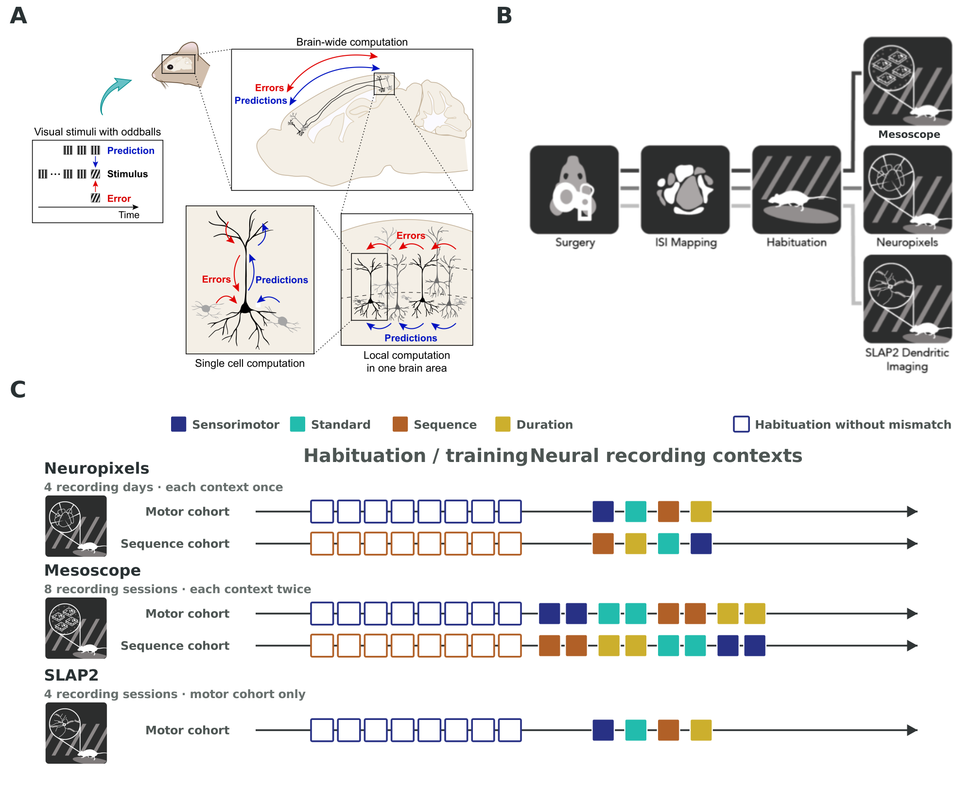
Figure 1:Distributed predictive-processing hypotheses motivate multimodal recordings. A, A visual sequence establishes an expectation (blue), whereas an unexpected oddball produces a prediction-error signal (red). Predictions and errors may be expressed through reciprocal brain-wide pathways, within local cortical populations, and across the dendritic and somatic compartments of individual neurons. B, To sample these nested scales within one standardized project, animals progressed from surgery through intrinsic-signal-imaging mapping and habituation before recording with mesoscope two-photon imaging, Neuropixels electrophysiology, or SLAP2 dendritic imaging. C, Five cohort timelines show eight outlined habituation and training sessions followed by filled neural-recording sessions. Neuropixels and mesoscope sampled motor- and sequence-habituated cohorts in opposite context orders. Neuropixels sampled every context once, whereas mesoscope repeated each context twice; SLAP2 sampled the motor-habituated cohort only.
The challenge of predictive processing research
Predictive processing theories propose that the brain continuously generates predictions about incoming sensory signals and updates its internal models when those predictions are violated. These prediction errors are thought to drive perception, learning, and behavior. While this framework has gained considerable theoretical support, significant conflicts persist in the experimental literature regarding the neural mechanisms that implement predictive computations.
Relationship to the companion review
This data release follows up a community review paper which synthesizes the theoretical motivations, identifies the key convergences and divergences in the predictive processing literature, and details the experimental hypotheses that this dataset was designed to test Aizenbud et al., 2026. Specifically, the dataset allows testing of two overarching alternative hypotheses: (H0) that different types of prediction errors involve fundamentally distinct neural mechanisms with specialized circuits for each type, or (H1) that a common computational principle underlies all mismatch responses, with apparent differences reflecting implementation variations.
What gap this dataset fills
A recent (May 6, 2026) database search on PubMed using the Boolean search: “predictive processing” OR “predictive coding”, returned more than 3,000 peer-reviewed publications (3,166). A thorough meta-analysis of such a large amount of scientific literature is arguably beyond the capability of any individual scientist. Recently, a group of more than 60 experts in the field thus aimed to collectively review this research corpus Aizenbud et al., 2026. A main finding of this collective effort was that the concept of predictive processing has given rise to multiple, loosely overlapping research fields that differ both in research methodology as well as experimental paradigms. That is, experimental studies on predictive processing range in scope from measurements of single neurons to full brain studies, giving rise to computational models that range from single synapses to large neuronal networks. And, at the same time, experimental studies on predictive processing use a large variety of different stimuli, giving rise to a variety of computational models that support some but not other paradigms. As a consequence, research on predictive processing has grown fragmented both methodologically and conceptually. This fragmentation produced a multitude of gaps in the research landscape that collectively impede coherent assessment of the current state of the art of predictive processing as a whole.
Our dataset was designed to fill these gaps by creating a bridge across both these dimensions (methods and stimuli) in an attempt to unify the divergent approaches. The overall aim is rigorous evaluation and study of predictive processing across experimental paradigms and neuroscientific methodologies. More specifically, as discussed below, we employed 4 of the most commonly used stimulus designs across 2 of the most commonly used techniques (electrophysiology and neuroimaging). On top of that, we added single vesicle glutamate imaging (SLAP2) to expand spatial coverage from multiple brain areas down to singular synaptic spines, or from multi-area computations down to single neuron computations. Each of these methodological modalities were performed in vivo using the same standardized experimental paradigm and stimuli (Figure 1).
Cross-context comparability
Existing studies of prediction errors typically employ only one class of mismatch stimulus (e.g., an orientation oddball or a visuomotor mismatch) in isolation, making it impossible to determine whether the observed neural responses reflect a general prediction error mechanism or a stimulus-specific computation. Our experimental design presents four distinct types of prediction violations (standard oddball, sensorimotor mismatch, temporal sequence mismatch, and duration mismatch) enabling direct comparison of mismatched responses across animals (Figure 2).
Large-scale, multi-modal population recordings
Previous datasets are typically limited to a single recording modality, preventing comparison of signals at different spatial and temporal scales. Our dataset combines Neuropixels electrophysiology (providing single-unit resolution across many brain regions simultaneously), mesoscope two-photon imaging (providing cell-type-specific calcium signals across VISp and VISlm, two visual areas in the mouse visual cortex), and SLAP2 imaging (providing subcellular dendritic recording in in the center of VISp). This multi-modal approach allows researchers to address questions about predictive processing at scales ranging from subcellular compartments to brain-wide networks.
Experimental design
Two cohorts design
To investigate whether prior experience with a specific predictive context influences neural responses to prediction violations, animals were divided into two cohorts that differed in their habituation experience and the order in which experimental sessions were presented. Both cohorts underwent all four mismatch session types, but the session experienced first (and for which animals had extensive prior habituation) differed between cohorts. This design enables within-animal comparison of mismatch responses across contexts, while the between-cohort comparison reveals how learned expectations from habituation shape these responses Aizenbud et al., 2026.
The motor cohort was habituated in a closed-loop visuomotor environment in which locomotion on a running disc controlled the phase of a vertical drifting visual grating stimulus that mimicked optic flow. During habituation (days 6–10, with session durations increasing from 8 to 48 min) and full-length training sessions (>1 h), animals experienced continuous closed-loop optic flow without any mismatch events.
The sequence cohort was habituated to passively view repeating sequences of drifting gratings (A–B–C–D–grey) without any mismatch events. During habituation (days 6–10, durations 8–48 min) and full-length training sessions (>1 h), animals viewed these sequences while freely running on the disc, which had no effect on the visual stimulus.
The motor cohort was recorded in the order sensorimotor mismatch, standard oddball, sequence mismatch, and duration mismatch. The sequence cohort was recorded in the order sequence mismatch, duration mismatch, standard oddball, and sensorimotor mismatch.
In both cohorts, the session that matched the habituation context was presented first, ensuring maximal learned expectation for the primary mismatch type. The remaining three sessions were presented in a counterbalanced order across cohorts. Each session was run in immediate succession: once for Neuropixels electrophysiology and twice for mesoscope two-photon calcium imaging, resulting in four or eight total recording sessions per animal. Given a limited throughput, experiments with the SLAP2 platform focused on the motor cohort. Each platform was used in a way that leverage their respective strengths: Experiments using the Mesoscope modality aimed to target the same exact population of neurons across all sessions types twice for a total of 8 cell-matched sessions; experiments using the Neuropixels modality were new probe insertions each day and aimed to record from the same areas (but not the same units) across all 4 types exactly once; experiments on the SLAP2 modality aimed to record the same neuron across all 4 sessions types exactly once. Across all modalities, those goals were met with pass/failure rates that are shared below. This cross-modality allocation is summarized in Figure 1C. QC-passing unit yields across the four Neuropixels recording days are summarized in Supplementary Figure 2.
Four predictive contexts
The four contexts tested violations of expected visual features (standard oddball), locomotion-linked visual feedback (sensorimotor mismatch), stimulus order (sequence mismatch), and stimulus timing (duration mismatch). Each context was embedded in a common session structure with matched control blocks and shared natural-movie and receptive-field stimuli. Trial tables were generated for each session and pseudo-randomized to vary deviant timing, while block order was held constant.
The shared within-session architecture and context-specific stimulus selection are summarized in Figure 2. Full session protocols and control-block parameters are described under Stimuli parameters in Methods.
Figure 2:Within-session architecture for cross-context comparison. A shows the common session sequence: a standard control precedes each context block and is repeated immediately afterward, followed by shared randomized, duration, open-loop, receptive-field, and zebra-movie blocks. B details the four contexts and the control and system-identification stimuli used to measure context-induced changes in response properties. Sources: pinned example tables, generator, Bonsai workflow, and public NWB intervals for electrophysiology and mesoscope.
The mismatch repeat count and session length were informed by the five published visual oddball paradigms compared in Supplementary Table 1. Those studies reported 10--144 required oddball repeats and total session durations ranging from 6 min to 2 h. We therefore set each 26-min context block to 1.35 mismatch events per minute for each of four deviant types (5.4/min combined), targeting approximately 35 repeats per deviant type and 140 mismatch events per context block. This placed per-deviant sampling within the published range while keeping the complete shared block sequence to approximately 71 min and applying the same event rate across all four predictive contexts.
Multimodal recording hardware
The three recording platforms sampled complementary spatial scales during the shared visual-stimulation paradigm (Figure 3). Six acute Neuropixels probes targeted distributed cortical and subcortical structures, while mesoscope two-photon calcium imaging sampled eight chronic imaging planes across VISp and VISlm. SLAP2 imaging targeted proximal and apical dendritic compartments of layer II/III pyramidal neurons in VISp. Recordings were collected in separate animals with modality-specific implants; the shared stimulus protocol, rather than simultaneous acquisition, provides the basis for comparisons across platforms. Acquisition and targeting procedures are described under Neuronal recording modalities.
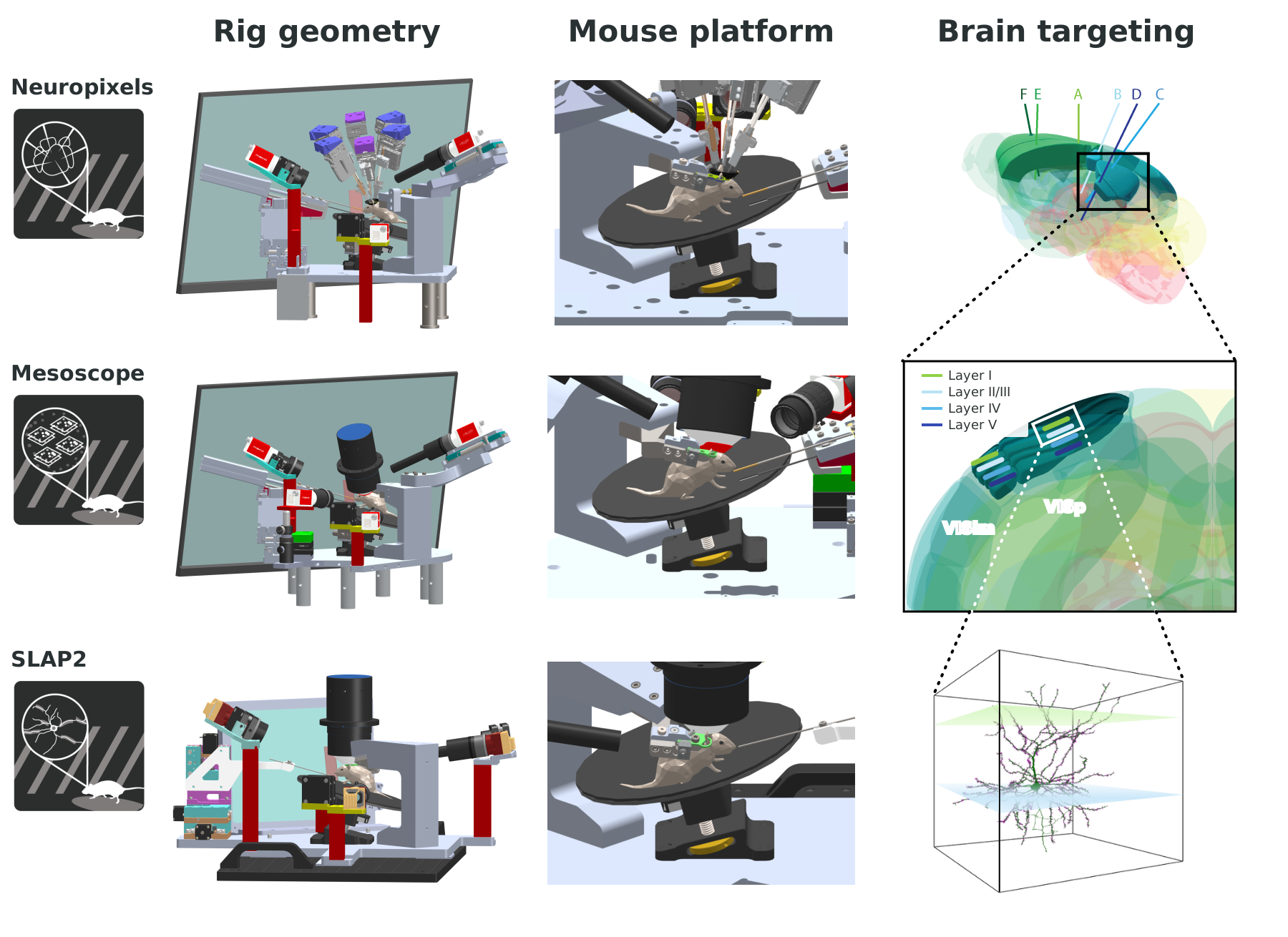
Figure 3:Multimodal recording hardware. Rows compare Neuropixels electrophysiology, mesoscope two-photon calcium imaging, and SLAP2 dendritic imaging. Columns show each rig geometry, the corresponding head-fixed mouse platform, and the brain-targeting strategy. Neuropixels uses six acute trajectories spanning cortical and subcortical structures; mesoscope uses eight chronic imaging planes across VISp and VISlm; and SLAP2 samples proximal and apical dendritic compartments in a layer II/III pyramidal neuron. The figure is reconstructed from nine native-resolution images extracted directly from the editable PowerPoint source.
Methods
Show complete Methods
Experimental animals
All animal procedures were approved by the Institutional Animal Care and Use Committee (IACUC) at the Allen Institute under protocol 2427 and conducted in accordance with NIH guidelines. Following surgery (see below), all mice were single-housed and maintained on a reverse 12-hour light cycle in a shared facility with room temperatures between 68º and 72ºF and humidity between 30 and 70%. All experiments were performed during the dark cycle. All mice in these experiments were given ad libitum access to food (regular or doxycycline diets) and water.
To systematically collect physiological data, we used standardized data collection and processing pipelines that were previously introduced de Vries et al., 2020Groblewski et al., 2020Durand et al., 2023Bennett et al., 2024Siegle et al., 2021. The data collection workflow progressed from surgical headpost implantation and craniotomy to retinotopic mapping of cortical areas using intrinsic signal imaging, in vivo recording of neuronal activity using various modalities (Neuropixels, Mesoscope two photon imaging, SLAP2 dendritic two-photon imaging), brain fixation and brain histology (see Figure 1). We describe each one of those steps in the dedicated sections below. As part of this workflow, all mice were trained on one of two possible cohorts: A motor cohort and a sequence cohort. Details of each cohort is described in the behavioral training section below. Both behavioral cohorts were recorded with the Neuropixels and Mesoscope recording modality. Only the motor cohort was used for SLAP2 experiments. Each modality (Neuropixels, Mesoscope, SLAP2) was recorded with separate mice as they had different, modality-specific brain implants.
Mesoscopic two-photon calcium imaging experimental animals
For experiments involving calcium imaging of GCaMP8s positive cells, male and female transgenic mice (n=14) with pan-neuronal cortical expression of GCaMP8s were used. Snap25-IRES-Cre Harris et al., 2014 was bred in-house and crossed with a GCaMP8s reporter line (Oi4), both of which are maintained on a C57BL/6J background. Snap25-IRES-Cre;Oi4 breeding sets consisted of heterozygous Snap25-IRES-Cre mice (JAX stock #023525) crossed with heterozygous or homozygous TIGRE2-RiboL1-jGCaMP8s-IRES-tTA2 (aka Oi4) mice (JAX stock #039267) Daigle et al., 2018Zhang et al., 2023. Experimental animals were heterozygous for both transgenes (full genotype Snap25-IRES2-Cre/wt;Oi4(TIT2L-jGCaMP8s-RiboL1-WPRE-ICL-IRES-tTA2-WPRE)/wt). Experimental mice show pan-neuronal expression patterns of GCaMP8s in Snap25-expressing cell populations. All mice (including breeders) were maintained on a 200 mg/kg rodent doxycycline diet (Bio-Serv; Flemington, NJ) to suppress tTA2 activity (and subsequent TRE2 promoter-driven expression) during development. Breeding cages were continuously maintained on a doxycycline diet. At weaning (~p20) mice with correct genotype were transferred to cages with standard chow for the remainder of the experiment (PicoLab 5L0D; Lab Diet, Richmod, IN). Despite limiting GCaMP8s expression during development with doxycycline the mice exhibited a sex-dependent reduction in survival rates at older age; at p200 males had a 72% survival rate while females had a 61% rate, n=123). We were unable to identify a clear, single cause for this reduced survival rate.
Neuropixels electrophysiology experimental animals
For experiments involving opto-tagging of inhibitory cells, male and female transgenic mice (n=17) expressing ChR2 in Cre-defined cell populations were used. Sst-IRES-Cre mice were bred in-house and crossed with an Ai32 channel rhodopsin reporter line, both maintained on a C57BL/6J background. Sst-IRES-Cre;Ai32 breeding sets consisted of heterozygous Sst-IRES-Cre mice (JAX stock #028864) crossed with homozygous Ai32(RCL-ChR2(H134R)_EYFP) mice (JAX stock #024109) Madisen et al., 2012Taniguchi et al., 2011. Experimental mice were heterozygous for both transgenes (full genotype Sst-IRES-Cre/wt;Ai32(RCL-ChR2(H134R)_EYFP)/wt). Cre+ cells from Ai32 lines are highly photosensitive, due to expression of Channelrhodopsin-2 Zhang et al., 2006.
SLAP2 experimental animals
For experiments involving simultaneous glutamate and calcium imaging, male and female wild-type C57BL/6J mice from JAX laboratory injected with Cre-dependent hSyn.FLEX.iGluSnFR4f.NGR and CAG.FLEX.RCaMP3 (or jRGECO1a) AAVs (serotype PHP.eB) were used. Sparse labeling was achieved via low titers (6E+8 vg/mL) of CaMKII-Cre virus. For experiments involving dendritic voltage imaging, male and female wild-type C57BL/6J mice from JAX laboratory injected with Cre dependent ASAP7 virus were used.
Surgery & cranial window procedure: two-photon calcium imaging experiments
A subset of mice received a headpost and cranial window surgery as previously described Groblewski et al., 2020de Vries et al., 2020. Headpost and cranial window surgery was performed on healthy male and female transgenic mice (p54-p80) weighing no less than 14 grams at time of surgery. Pre-operative injections of dexamethasone (3-4.2 mg/kg, S.C.) and ceftriaxone (100-125 mg/kg, S.C.) were administered at 1h before surgery. Additionally, carprofen was administered for pain management (5-10 mg/kg, S.C.), and atropine was administered to suppress bronchial secretions and regulate heart rhythms (0.02-0.05 mg/kg, S.C.). Mice were initially anesthetized with 2-4% isoflurane and placed in a stereotaxic frame (Model# 1900, KOPF; Tujunga, CA), and isoflurane levels were maintained at 1.0-2.0% for surgery. An incision was made to remove skin, and the exposed skull was levelled with respect to pitch (bregma-lambda level), roll and yaw. The stereotax was zeroed at lambda using a custom headframe holder equipped with a stylus affixed to a clamp-plate. The stylus was then replaced with the headframe to center the headframe well at 2.8 mm lateral and 1.3 mm anterior to lambda. The headframe was affixed to the skull with white dental cement (C&B Metabond; Parkell; Edgewood, NY) and once dried, the mouse was placed in a custom clamp to position the skull at a rotated angle of 23° such that the visual cortex was horizontal to facilitate creation of the craniotomy. A circular piece of skull 5 mm in diameter was removed, and a durotomy was performed. A glass coverslip (cut from a single piece of glass to obtain a “stacked” appearance that consisted of a 5 mm diameter “core” and 7 mm diameter “flange”), was cemented in place with Vetbond (3M; St. Paul, MN). Dental cement was then applied around the cranial window inside the well to secure the glass window, and subsequently covered with black tempura paint to reduce glare during imaging. The mouse was given 1.0-1.5mL Lactated Ringers Solution (LRS) to help recover from the surgery and replace lost fluids. Post-surgical brain health was documented using a custom photo-documentation system and animals were assessed one, two, and seven days following surgery for overall health (bright, alert and responsive), cranial window clarity and brain health.
Surgery & cranial window procedure: Neuropixels experiments
A subset of the mice received the SHIELD surgical procedure, which has previously been described Bennett et al., 2024. The SHIELD procedure was performed on healthy male and female transgenic mice (p53-p139) weighing no less than 14 grams at time of surgery. Pre-operative injections of dexamethasone (3-4.2 mg/kg, S.C.) and ceftriaxone (100-125 mg/kg, S.C.) were administered 1 h before surgery to reduce swelling and postoperative pain. Additionally, carprofen (5-10 mg/kg, S.C.) was administered for pain management, and atropine (0.02-0.05 mg/kg, S.C.) was administered to suppress bronchial secretions and regulate heart rhythms. Mice were initially anesthetized with 2-4% isoflurane and placed in a stereotaxic frame (Model# 1900, KOPF; Tujunga, CA). Isoflurane levels were maintained at 1.0-2.0%, and body temperature was maintained at 37.5°C for the duration of the surgery. An incision was made on the dorsal surface of the skull, and skin was removed in a teardrop shape, exposing the rostral rhinal vein between the eyes, the dorsal surface of the parietal and occipital skull plates, and stopping where the neck muscle begins to attach to the back of the skull. Next, the periosteum was removed from the skull surface to improve adhesion of the cement to the skull and prevent future scabbing and infection. Starting posterior of the left eye, angled forceps were used to separate cheek muscle from the skull, as well as connective tissue and muscle above the left ear. The cheek muscle was then pulled away from the skull and is stretched out so that it makes a seal with the left lateral portion of the well. The exposed skin (and any exposed soft tissue such as the cheek muscle) was then sealed with Vetbond, and the exposed skull was leveled with respect to pitch, roll, and yaw. Once the skull was leveled, bregma was identified using the custom bregma stylus. Without moving the stereotaxic arm in X or Y, the stylus was replaced with a custom “tracer” that provides a guide for marking the craniotomy with respect to bregma. A #11 scalpel blade (or forceps) was used to etch a faint line in the skull around the tracer, which was then replaced with a shallow trench by lightly drilling without breaking through the skull (NeoBurr EF4). After etching was complete, the tracer was replaced with the headframe, which was then lowered in Z to make contact with the skull. Next, dental cement (C&B Metabond, Parkell) was used to attach the headframe to the skull. Once the cement hardened, the headframe was clamped into a custom frame, and the craniotomy and durotomy were performed. After sterilization, a custom implant was then lowered into the craniotomy. To provide a surface that can be glued to the skull, a flange on the implant extends beyond the cranial window and sits directly on the bone, where it was sealed with Vetbond and attached to the skull Once dry, the vetbond was covered with metabond to further secure the implant to the skull. The inner part of the implant sits on the brain surface. Any areas of exposed skull were then covered with cement. Any white cement on the inside of the well was coated with a layer of black tempura paint to reduce glare during ISI imaging. The mouse was given 1.0-1.5mL Lactated Ringers Solution (LRS) to help recover from the surgery and replace lost fluids. After removing the mouse from anesthesia, but prior to it waking up, a photo-documentation image was acquired. Finally, a removable plastic cap was placed over the well to protect the coated implant from cage debris, and the mouse was returned to its home cage for recovery. Over the following 7-14 days, mice were monitored regularly for overall health, cranial window clarity, and brain health.
Surgery & cranial window procedure: SLAP2 experiments
A subset of mice received the SLAP2 Visual Cortex laser level procedure. The SLAP2 Visual Cortex laser level procedure was performed on healthy male and female transgenic mice (p53-p139) weighing no less than 14 grams at time of surgery. This is a variation on the Visual Cortex surgery used for the mesoscope experiments. To achieve single cell resolution the optimal angle for the SLAP2 microscope is as close to perpendicular to the craniotomy coverslip as possible. To facilitate this the headframe was attached after the coverslip was secured. This allowed the headframe to be installed on a consistent plane relative to the coverslip, ensuring proper interfacing between the craniotomy and SLAP2 microscope objective. Pre-operative injections of dexamethasone (3-4.2 mg/kg, S.C.) and ceftriaxone (100-125 mg/kg, S.C.) were administered 1 hour before surgery to reduce swelling and postoperative pain and protect against infection. Additionally, carprofen (5-10 mg/kg, S.C.) was administered for pain management, and atropine (0.02-0.05 mg/kg, S.C.) was administered to suppress bronchial secretions and regulate heart rhythms. Mice were initially anesthetized with 4% isoflurane and placed in a stereotaxic frame (Model# 1900, KOPF; Tujunga, CA). Isoflurane levels were maintained at 1.0-2.0%, and body temperature was maintained at 37.5°C for the duration of the surgery. An incision was made on the dorsal surface of the skull. Skin was removed in a teardrop shape; exposing the rostral rhinal vein between the eyes, the dorsal surface of the parietal and occipital skull plates and stopping where the neck muscle begins to attach to the back of the skull. Next, the periosteum was removed from the skull surface to improve adhesion of the cement to the skull and prevent future scabbing and infection. Starting posterior to the left eye, angled forceps were used to separate cheek muscle from the skull, as well as connective tissue and muscle above the left ear. The cheek muscle was then pulled away from the skull and stretched out so that it makes a seal with the left lateral portion of the well. The exposed skin, and any exposed soft tissue such as the cheek muscle, was sealed with Vetbond (3M; St. Paul, MN). The 5mm craniotomy “tracer” provided a guide for marking the craniotomy and was centered at 2.8 mm lateral and 1.3 mm anterior to lambda. Forceps were used to etch a faint line in the skull around the tracer. Using the drill (NeoBurr EF4), without breaking through the skull, the etch was then replaced by a shallow trench. The mouse was rotated clockwise approximately 23 degrees to create a level surface to drill on and help angle the coverslip to accurately interface perpendicularly with the SLAP2 microscope. A well was created with a silicone polymer (Body Double Fast; Smooth-On; East Texas, PA) large enough to encompass the craniotomy and bregma. Craniotomy and durotomy were then performed. The mouse was rotated back 23 degrees counterclockwise for virus injection. A Nanoject III (Drummond; Broomall, PA) was then zeroed at bregma, and virus was injected with a beveled pipette at 3.1 mm lateral, 3.1 mm posterior to and at 3.1 mm lateral, 3.9 mm posterior to bregma, at depths of 0.3 mm and 0.6 mm below surface of the cortex for each point. The mouse was rotated back clockwise approximately 23 degrees to return the craniotomy to an approximately leveled plane relative to pitch, roll, and yaw. A glass coverslip (cut from a single piece of glass to obtain a “stacked” appearance that consisted of a 5 mm diameter “core” and 7 mm diameter “flange”), was lowered into the craniotomy. The 2mm flange was cemented in place with Vetbond. A custom in-house laser leveling tool was used to level the coverslip so that it was perpendicular to the stereotaxic arm. The mouse skull was turned back 23 degrees counterclockwise, and pitch was raised 6 degrees to keep the coverslip in a parallel plane relative to the headframe. This allowed for proper interfacing of the glass coverslip and the SLAP2 microscope when the mouse was head fixed in the headframe. Using the stereotaxic arm, a headframe was lowered onto the skull and secured in place with clear dental cement (C&B Metabond; Parkell; Edgewood, NY), covering all remaining exposed skull. Black tempura paint was applied on top of the clear cement outside the headframe to reduce light leaks. The mouse was given 1.0-1.5mL Lactated Ringers Solution (LRS) to help recover from the surgery and replace lost fluids. After removing the mouse from anesthesia, prior to it waking up, post-surgical brain health was documented using a custom photo-documentation system. Animals were assessed on days one, two, and seven following surgeries for overall health (bright, alert and responsive), cranial window clarity and brain health.
Intrinsic signal imaging / retinotopic mapping
Intrinsic signal imaging (ISI) measures the hemodynamic response of the cortex to visual stimulation across the full field of view. This retinotopic mapping represents the spatial relationship between the visual field and cortical locations within each visual area. For both Neuropixels and Mesoscope two-photon imaging experiments, retinotopic maps were used to delineate functionally defined visual area boundaries and to guide targeting of in vivo two-photon calcium imaging to retinotopically defined locations in primary and secondary visual areas.
Animal preparation
For every ISI imaging session, mice were lightly anesthetized with 1–1.4% isoflurane delivered via a SomnoSuite system (model 715; Kent Scientific, CT, USA) at a flow rate of 100 mL/min, supplemented with ~95% O₂ (Pureline OC4000; Scivena Scientific, OR, USA). Lubricating eye ointment (Lacri-Lube; Refresh) was applied to maintain corneal hydration and clarity during anesthesia. Mice were positioned on a lab jack and head-fixed such that the cranial window was normal to the imaging axis. The head frame and clamping mechanism ensured consistent positioning of the eye relative to the stimulus monitor across experiments.
Image acquisition system
To map retinotopic organization and standardize data acquisition, a custom ISI system coupled to visual stimulation was used. The cortical surface was illuminated with a ring of independently controlled LEDs, including green (peak λ = 527 nm, FWHM = 50 nm; Cree Inc., C503B-GCN-CY0C0791) and red (peak λ = 635 nm, FWHM = 20 nm; Avago Technologies, HLMP-EG08-Y2000) wavelengths mounted on the objective. A tandem lens configuration (Nikon Nikkor 105 mm f/2.8 rear lens and Nikon Nikkor 35 mm f/1.4 front lens) provided 3.0× magnification (M = 105/35). The back focal plane of the front lens was positioned adjacent and coplanar to the cranial window (working distance: 46.5 mm). A bandpass filter (Semrock FF01-630/92 nm) was used to preferentially transmit longer-wavelength reflectance signals while minimizing contamination from the stimulus monitor and ambient light.
Image acquisition and illumination were controlled via custom Python software. Images were acquired using an Andor Zyla 5.5 10-tap sCMOS camera at 40 Hz, with frame timing governed by the camera’s 40 MHz hardware clock. Image acquisition and stimulus presentation were synchronized via hardware triggering from a National Instruments digital I/O board. Raw images (2560 × 2160 pixels, 16-bit) were spatially (4×4) and temporally (4×) binned to yield 640 × 640 pixel frames at 10 Hz with 32-bit dynamic range and an effective pixel size of 10 µm.
Intrinsic imaging visual stimulus
The lambda–bregma axis of the skull was oriented at a 30° pitch relative to horizontal, corresponding to an eye position approximately 60° lateral to the midline and 20° above the horizon Oommen & Stahl, 2008. A 24″ monitor was positioned 10 cm from the right eye to maximize visual field coverage. The monitor was rotated 30° relative to the dorsoventral axis and tilted 70° relative to the horizon to maintain perpendicularity to the optic axis.
The visual stimulus consisted of a drifting bar containing a contrast-reversing checkerboard pattern on a gray background. The bar swept across the four cardinal directions at 0.1 Hz, with 10 repetitions per direction Kalatsky & Stryker, 2003. The bar measured 20° × 155°, with individual checker squares of 25°. Stimuli were spatially warped to approximate a spherical visual field projection on a flat display Marshel et al., 2011.
Image acquisition and processing
A high-resolution image of the cortical vasculature was first acquired under green illumination to serve as a fiducial reference. The imaging plane was then defocused 500–1500 µm below the surface to capture intrinsic signals. Up to 10 ISI time series were collected per experiment.
Time series were preprocessed by removing the time-averaged pixel intensity (DC component) to improve signal-to-noise ratio. A discrete Fourier transform (DFT) was computed at the stimulus frequency. Phase maps were generated from the phase angle of the DFT and used to map visual field position onto cortical coordinates. Sign maps were derived by computing the sine of the angle between the gradients of the altitude and azimuth phase maps. Final sign maps were averaged across at least three time series (minimum of 30 sweeps per direction).
Automated sign map segmentation and annotation
For each experiment, visual field sign maps were segmented into distinct visual areas using an automated algorithm (adapted from Garrett et al., 2014). Segmentation was based on three criteria: (1) each area contains a uniform visual field sign, (2) each area represents a unique (non-redundant) portion of visual space, and (3) adjacent areas with the same sign exhibit redundant visual field representations.
Eccentricity and target map generation
Eccentricity maps were computed relative to the center of visual space (0° azimuth, 0° altitude). When the eye is properly aligned, this point corresponds approximately to the anatomical center of V1. The eccentricity at the V1 centroid was used as a quality control metric to identify experiments with significant eye misalignment (>15°).
To define target regions for two-photon imaging, eccentricity maps were thresholded to include locations within 10° of the V1 center. These targeting maps were overlaid onto vasculature images to provide fiducial landmarks for aligning imaging fields across sessions and ensuring retinotopic consistency.
ISI quality control
Quality control of ISI-derived maps consisted of four steps:
Brain surface and vasculature images were inspected before and after acquisition for clarity, focus, and cranial window positioning.
Individual trials were evaluated for sufficient visual coverage, continuity of phase maps, localization of amplitude maps, and expected sign map organization. Only trials meeting these criteria were included (minimum of three trials).
Automated segmentation was required to identify at least six visual areas (VISp, VISlm, VISrl, VISal, VISam, VISpm).
Final maps were assessed for visual field coverage (35–60° altitude, 60–100° azimuth), minimal bias (<10° range imbalance), alignment of the retinotopic center with the V1 centroid, and minimum V1 area (>2.8 mm²).
Behavioral training
Mice were trained in individual sound-attenuating enclosures arranged in clusters. Each enclosure was arranged similarly to that of the mesoscope two-photon microscope, SLAP2 two-photon imaging microscope and the Neuropixels rigs. A 24” LCD monitor was positioned 15 cm from the mouse’s right eye, with the sagittal axis of the head parallel to the screen. A registered headframe clamp was attached to a behavior stage equipped with kinematic mounts to ensure repeatable placement of the stage in the enclosure. Each stage consisted of a fixed-position headframe clamp and adjustable running wheel. Enclosures were equipped with a camera coupled with IR illumination to monitor mouse activity. Those videos were recorded but kept temporarily on disk.
Animals received a 2-week training procedure following a previously published head-fixation habituation protocol de Vries et al., 2020.
Habituation to handling and head-fixation was performed for five days: On days 1-2 mice were removed from the home cage and gently handled for 1-2 min. On days 3-5 mice were removed from the home cage and handled for 1-2 min, then head-fixed by securing the headframe in the behavior stage clamping mechanism. The stage was then placed in the lit behavior enclosure for 5-10 min.
Passive behavior training was then performed to habituate mice to extended periods of head-fixation and expose the mice to visual stimuli. On days 6-10 mice were removed from the home cage and handled for 1-2 min. Mice were then head-fixed to the behavior stage and the stage was placed in the behavior enclosure. A set of full-screen stimuli was displayed for increasing periods. Visual stimuli were displayed for increasing durations of 8, 18, 28, 38, and 48 min on days 6 through 10, respectively.
The habituation protocol included two cohorts of mice. (1) The sequence cohort passively viewed a repeating sequence of four drifting gratings (90°–45°–0°–45°) followed by a grey inter-sequence interval, without any mismatch events. Each element was presented for 250 ms, and gratings were full-field (0.04 cpd, 2 Hz temporal frequency, 100% contrast). Animals were free to walk and rotate the disc beneath their body; however, disc rotation had no effect on the stimuli presented on the screen. This established a learned expectation for the sequential structure. (2) The motor cohort was habituated in a closed-loop paradigm in which locomotion on the running disc controlled the phase of a full-field sinusoidal grating (0° orientation, 0.04 cpd) via a rotary encoder. This configuration approximated natural visual flow, such that forward locomotion produced corresponding backward grating motion consistent with that experienced by a freely moving mouse. No mismatch events were presented during any habituation sessions in either cohort. The full-length habituation sessions additionally included control blocks (standard control, sequential control, jitter control, open-loop prerecorded, natural movie, and receptive field mapping) identical to those used in the experimental sessions, further habituating the animals to the full session structure.
Visual stimulation
All visual stimuli were generated using BonVision Lopes et al., 2021, an open-source visual environment package running within the Bonsai reactive programming framework Lopes et al., 2015. For behavior training, Neuropixels recordings and mesoscope imaging, stimuli were rendered at 60 Hz and displayed on a gamma-calibrated ASUS PA248Q LCD monitor (1920 × 1200 pixels, 55.7 cm wide, 60 Hz refresh rate) positioned 15 cm from the animal’s right eye (see Figure 1). A spherical warping correction (BonVision SphereMapping) was applied to all stimuli to compensate for the close viewing distance and flat display geometry, ensuring that apparent size, speed, and spatial frequency were constant across the visual field as seen from the mouse’s perspective. The monitor subtended 120° × 95° of visual space. Mean luminance was 50 cd/m². Stimulus timing was synchronized to neural recordings via a photodiode placed on a sync square region of the monitor that alternated between black and white every 60 frames, and via digital synchronization pulses sent to a National Instruments digital board. The full stimulus code, Bonsai workflow, and parameter files are available on the project’s GitHub repository (https://
For each session, a stimulus table (CSV file) was generated programmatically by a Python script (generate_experiment_csv.py) using a session-specific random seed derived from the session UUID and timestamp, ensuring unique trial sequences across sessions while maintaining reproducibility. This CSV table specified all trial parameters (orientation, spatial frequency, temporal frequency, contrast, duration, delay, position, phase, trial type, and block membership) and was read by the Bonsai workflow (generic_oddball.bonsai) to drive stimulus presentation in sequence.
In the sensorimotor mismatch context, the phase of the drifting grating was coupled to the angular position of the running disc via a rotary encoder. The wheel-to-visual coupling was computed as: phase (radians) = 2π × R × θ / tan(1/f × π/180), where R is the wheel radius-to-screen ratio (0.36), θ is the wheel angle in degrees, and f is the spatial frequency (0.04 cpd). This coupling was calibrated so that the resulting visual flow approximated the optic flow a freely moving mouse would experience during forward locomotion.
Stimuli parameters
All drifting grating stimuli shared the following base parameters unless otherwise specified: spatial frequency 0.04 cpd, temporal frequency 2 Hz, 100% contrast, sinusoidal luminance profile, full-field extent (360° diameter with spherical correction). For the standard oddball, sequence mismatch, and duration mismatch sessions, gratings drifted at a fixed temporal frequency of 2 Hz. For the sensorimotor mismatch session, the grating phase was updated at 30 Hz (every other video frame) based on wheel rotation, with temporal frequency set to 0 in the stimulus table (wheel-controlled mode). Oddball/mismatch events occurred at a rate of 1.35 per minute per deviant type (5.4/min total across four deviant types) in all session types. The four session types and shared control blocks are described below.
Session type 1: Standard oddball
Full-field sinusoidal drifting gratings were presented in a classical oddball paradigm. The standard stimulus (0° orientation, 0.04 cycles per degree, 2 Hz temporal frequency, 100% contrast) was presented with high probability, with each trial consisting of a 343 ms stimulus presentation followed by a 343 ms grey inter-stimulus interval (686 ms total trial duration). Deviant stimuli occurred randomly at a combined rate of 5.4 per minute (1.35/min per type) and included: orientation deviants at 45° and 90°, a halt deviant (temporal frequency set to 0, producing a stationary grating), and an omission deviant (contrast set to 0, producing a blank screen).
Session type 2: Sensorimotor mismatch
Optic flow was coupled to the animal’s locomotion on the running disc, creating a closed-loop visuomotor environment. A full-field sinusoidal grating (0° orientation, 0.04 cpd) was displayed with its phase updated at 30 Hz based on wheel rotation. The coupling gain was set such that the visual flow was consistent with that experienced by a freely moving mouse. Mismatch events were introduced by transiently decoupling visual flow from locomotion for 343 ms. Mismatch types (each at 1.35/min) included: motor halt (temporal frequency set to 0, freezing grating motion despite continued locomotion), motor omission (contrast set to 0, removing the grating entirely), and motor orientation changes (grating orientation shifted to 45° or 90° while drifting at 2 Hz independent of the wheel). A minimum interval of 2 s separated consecutive mismatch events, with a 5 s buffer at the start and end of the block.
Session type 3: Sequence mismatch
Animals were presented with repeating five-element sequences of drifting gratings. Each sequence consisted of four oriented gratings (90°–45°–0°–45°) followed by a grey inter-sequence interval with each element presented for 250 ms, yielding a total sequence duration of 1.25 s. All gratings were full-field (0.04 cpd, 2 Hz temporal frequency, 100% contrast). Mismatch events were introduced by substituting the third element (normally 0°) of a sequence at a combined rate of 5.4 mismatch sequences per minute. Mismatch types included: orientation substitution to 45° (producing a repeated element where a change was expected), orientation substitution to 90° (introducing a novel orientation), halt (stationary grating), and omission (blank screen at the substitution position).
Session type 4: Duration/temporal mismatch
Full-field sinusoidal drifting gratings (0° orientation, 0.04 cpd, 2 Hz temporal frequency, 100% contrast) were presented with a standard trial structure of 343 ms stimulus followed by a 343 ms delay (686 ms total). Temporal prediction violations were introduced by altering the inter-stimulus delay while keeping the stimulus duration constant. Deviant delays included 150 ms (shorter than expected), 500 ms, and 1000 ms (longer than expected), each occurring at 1.35/min. Omission deviants (contrast = 0) were also included at 1.35/min.
Shared session design
All four session types shared an identical set of control blocks presented before and after the main mismatch block, enabling cross-session normalization and quality assessment. Each session comprised the following blocks in order:
Standard control block (6.4 min): 14 grating orientations (spaced every 22.5° from 0° to 315°) plus omission and halt trials, each repeated multiple times and presented in shuffled order. Each trial used the standard 343 ms stimulus + 343 ms delay structure (0.04 cpd, 2 Hz, 100% contrast, full-field). This block provides orientation tuning curves and adaptation-free baselines.
Main mismatch block (26 min): The session-specific mismatch paradigm (standard oddball, sensorimotor, sequence, or duration mismatch, as described above).
Standard control block (6.4 min): A repeat of the first control block, enabling assessment of response stability over the session.
Sequential control block (4.7 min): The same 14 orientations plus omissions and halts as in the standard control block, but presented with 250 ms duration (matching the temporal structure of the sequence mismatch paradigm) and shuffled randomly without sequential structure. This serves as a non-sequential baseline for the sequence mismatch session.
Jitter (duration) control block (6.4 min): Gratings (0° orientation, standard parameters) presented with seven different inter-stimulus delays (150, 343, 500, 750, 1000, 1500, and 914 ms), each repeated uniformly across the block, plus omission trials. This provides a matched-stimulus baseline for the duration mismatch session, where all delays occur with equal probability.
Open-loop prerecorded block (6.4 min): A shared pre-recorded wheel-derived phase trajectories (sampled at 30 Hz from previous running sessions) drove the grating phase in open loop, replicating naturalistic visual flow patterns without actual closed-loop coupling. Motor mismatch events (orientation changes, halts, and omissions, each at 1.35/min) were injected into this playback, providing a sensorimotor mismatch control condition where the animal’s locomotion does not match the visual flow.
Natural movie block (10 min): A naturalistic “zebra noise” movie (120° × 95° visual field, 30 fps, 300 s duration, presented twice) was displayed Skriabine et al., 2026. This stimulus serves as a shared reference for cross-session and cross-modality comparison, and provides a rich stimulus for characterizing neural response properties.
Receptive field mapping block (5 min): A small drifting grating patch (20° diameter, 0.08 cpd, 4 Hz temporal frequency, 80% contrast) was presented at 81 positions on a 9 × 9 grid spanning ±40° of visual space in 10° steps. Three orientations (0°, 45°, 90°) were tested at each position with 5 repeats, using 250 ms presentations. This block enables estimation of spatial receptive fields for individual neurons.
Neuronal recording modalities
Neuropixels extracellular electrophysiology
Habituation to the Neuropixels rigs.
Prior to the first recording, mice were habituated to the Neuropixels rigs every day for a week. These sessions were similar to the recording session in length but did not include oddballs. There were 2 cohorts of mice, one exposed to motor stimuli and the other to the sequence stimuli (see stimuli description).
Implant design for recordings
The implant was designed as stated in the surgery section and was described previously Bennett et al., 2024. Briefly, we created a CAD file with holes strategically placed above the areas of interest for our study (see Supplementary Figure 1). Some hole coordinates have been previously validated to allow targeting of areas such as the center of VISp, and other hole coordinates were derived from publications, such as VISa Lyamzin & Benucci, 2019. Hole positions were adjusted using Pinpoint Birman et al., 2023. Note that the placement of the implant on the brain can vary slightly due to mouse-to-mouse variability and surgical precision. The coordinates of holes were referenced from bregma; their diameters and intended target areas are represented in Supplementary Figure 1.
SORTA-Clear plug removal and agarose application
To prepare the brain for recording, the SORTA-Clear coating over the implant is removed and replaced with a temporary layer of Kwik-Cast (World Precision Instruments). The mouse is anesthetized with isoflurane (5% induction, 1-2% maintenance, 100% O2) and eyes protected with ocular lubricant (I-DROP, VetPLUS). Body temperature is maintained at 37.5°C (TC-1000 temperature controller, CWE, Incorporated). The well is cleaned of any debris using ethanol swabs. Then, the inside of the well surrounding the SORTA-Clear plug is painted with white Metabond to improve visibility during probe insertion. Once the Metabond is dry, the well is flooded with enough ACSF to completely submerge the SORTA-Clear sheet, which is then removed with small forceps, starting at the anterior or posterior end of the sheet and peeling gently to remove it in one piece. Once the SORTA-Clear sheet is completely detached from the implant, the edges of implant holes are tested with small forceps to ensure all holes are free of SORTA-clear or debris. ACSF is removed from the well using Sugi spears (Kettenbach) and the well is filled with Kwik-Cast. Once the Kwik-Cast is fully dry, a plastic protective cap is secured on the well to protect against debris and the mice are returned to their home cage. This preparation is generally performed Fridays for recordings on Mondays to avoid using isoflurane on the day of experiment.
Head fixation.
On the day of recording, the mouse is removed from its home cage and clamped to the running wheel on the experimental rig. Wheel height is adjusted as needed for each mouse. Once head-fixed, the protective well cap and Kwik-Cast layer are removed. The ground wire is tucked into the side of the well and any excess debris cleaned using a Sugi spear or cotton tipped applicator. Approximately 0.2ml of agarose (4%: 0.4 g of BioRad Low Melt and 0.4 g of Sigma agarose high electroendosmosis in 20.2 ml ACSF Durand et al., 2023 is applied in a smooth layer over the entire implant surface and ground wire. After popping any large bubbles, the agarose is allowed to set for ∼10 seconds. To prevent the agarose from drying out during the experiment, a layer of silicon oil is applied over exposed agarose with a toothpick. At the end of the experiment, the agar is removed and replaced with Kwik-Cast.
The 3D-printed protective cone was then lowered to prevent the mouse’s tail from striking the probes. An infrared dichroic mirror was placed in front of the right eye to allow the eye-tracking camera to operate without interference from the visual stimulus.
Grounding.
A 32 AWG silver wire (A-M Systems) is epoxied to the headframe during the implant surgery and served as the ground connection. The wire is pre-soldered to a gold pin embedded in the headframe well, which mates with a second gold pin on the protective cone. This second gold pin is connected to both the behavior stage and the probe ground. Prior to the experiment, the brain-to-probe ground path is checked using a multimeter. The reference connection on the Neuropixels probes is permanently soldered to ground using a silver wire, and all recordings are made using the tip reference configuration. The headstage grounds (which are contiguous with the Neuropixels probe grounds) are connected with 36 AWG copper wire (Phoenix Wire). All probes are connected in parallel to animal ground.
Neuropixels probes
All neural recordings were carried out with Neuropixels 1.0 probes Jun et al., 2017, as previously described Siegle et al., 2021Durand et al., 2023. The 384 electrodes closest to the tip are used, providing a maximum of 3.84 mm of tissue coverage. The signals from each recording site are split in hardware into a spike band (30 kHz sampling rate, 500 Hz highpass filter) and a Local Field Potential (LFP) band (2.5 kHz sampling rate, 1000 Hz lowpass filter). Our goal was to insert six probes into the same mouse’s brain on each of 4 consecutive days. To distinguish the paths of these different penetrations, we use two dyes, CM-DiI (1 mM in ethanol; ThermoFisher Product #V22888) on day 1 and 2 and CM-DiD (1mM in ethanol; AAT Bioquest catalogue number 22060) on day 3 and 4. The probes are coated with dye before recordings by immersing them at least 3mm into a well filled with dye. Each probe are dipped five times to ensure adequate coating.
Neuropixels probe insertion
Our custom experimental rig can insert up to six Neuropixels probes simultaneously (see Figure 3). Each probe is mounted on a separate 3-axis micromanipulator with a 15 mm travel range (New Scale Technologies, Victor, NY). Probes are driven to their target holes and lowered to the surface of the brain while the experimentalist monitores a camera feed to avoid vasculature and watches real-time signals on the OpenEphys GUI to identify activity indicative of the brain surface. If the probe need adjustment when attempting to insert (e.g. to avoid vessels), the probe are completely retracted out of the silicon oil to prevent probe bending. Once all probes reach the brain surface, each probe is zeroed and set to insert 3100 μm deep at 200 μm/min and then retracted 100 μm to their final depths to reduce tissue compression and subsequent electrode zdrift relative to the brain. Once all probes reach their final depth, the probes are allowed to settle for ∼30 minutes, and a photo documentation of the inserted probes is captured. Sometimes a probe can not be inserted into its assigned hole, failures are generally due to dura regrowth. Overall, we achieved a penetration success of 5.8 probes per session.
Data acquisition and synchronization.
Neuropixels data is acquired at 30 kHz (spike band) and 2.5 kHz (LFP band) using the Open Ephys GUI Siegle et al., 2017. Gain settings of 500× and 250× are used for the spike band and LFP band, respectively. Probes are connected to a PXIe card inside a National Instruments chassis.
Videos of the eye, body and face are acquired at 60 Hz. The angular velocity of the running wheel is recorded at the time of each stimulus frame, at approximately 60 Hz. Synchronization signals for each frame are acquired by a dedicated computer with a National Instruments card acquiring digital inputs at 100 kHz, which is considered the master clock. A 32-bit digital ‘barcode’ is sent with an Arduino Uno (SparkFun DEV-11021) every 30 s to synchronize all devices with the neural data. Each Neuropixels probe has an independent sample rate between 29,999.90 Hz and 30,000.31 Hz, making it necessary to align the samples offline to achieve precise synchronization. The synchronization procedure uses the first matching barcode between each probe and the master clock to determine the clock offset, and the last matching barcode to determine the clock scaling factor.
To synchronize the visual stimulus to the master clock, a silicon photodiode (PDA36A, Thorlabs) was placed on the stimulus monitor above a “sync square” that alternated between black and white every 60 frames.
Stimulus Monitor
We lower a black curtain over the front of the rig, placing the mouse in complete darkness except for the visual stimulus monitor. Visual stimuli are generated using custom scripts based on PsychoPy9 and are displayed using an ASUS PA248Q LCD monitor, with 1,920 × 1,200 pixels (55.7 cm wide, 60 Hz refresh rate). Stimuli are presented monocularly, and the monitor is positioned 15 cm from the right eye of the mouse and spans 120° × 95° of visual space before stimulus warping. Each monitor is gamma corrected and has a mean luminance of 50 cd m−2. To account for the close viewing angle of the mouse, a spherical warping is applied to all stimuli to ensure that the apparent size, speed and spatial frequency were constant across the monitor as seen from the mouse’s perspective.
Probe removal and cleaning
After each experiment, the probes are retracted from the brain at a rate of ~3000μm/min and the mouse is removed from head fixation and returned to its home cage. If another recording session is to occur the same day, the probes are then immersed in a well of freshly made 1% Tergazyme mixed with agarose for 5 minutes to remove excess residue, followed by immersion in 1% Tergazyme for 30 minutes, immersion in Milli-Q water for 25 minutes, and dipped in 100% isopropyl alcohol for 1 minute. After the last recording session of the day, the probes are immersed in a well of freshly made 1% Tergazyme for ~12 hours.
Quality Control for Neuropixels recording sessions
Possible QC failure can come from these cases: white foam buildup on the edge of the eye covering the pupil, software failures compromising critical data streams, visual stimulus synchronizing failure, cortical bleeding or compromised brain health resulting in low unit activity and/or atypical visual responses, gap in data acquisition and discovery of purulent material over right hemisphere during ex-vivo imaging. Out of a total of 56 sessions, 12 are excluded for eye foam.
Optotagging protocol
At the end of every experiment, an optotagging protocol is run during which the cortical surface is stimulated with blue light. In Sst-IRES-Cre/wt;Ai32(RCL-ChR2(H134R)_EYFP)/wt mice, this protocol allowes us to identify putative Sst+ cortical interneurons by an increase in spiking activity time-locked to laser stimulation (and consequent ChR2 activation). Blue light is delivered by a 473 nm laser (Laser Quantum, model Ciel or Cobolt model 06-MLD). The light source is coupled to a 400 μm diameter fiber optic cable (Thorlabs) or bifurcated fiber bundle (Thorlabs, BFYL4LF01), with the tip(s) positioned such that blue light illuminates the entire cranial window. Two types of stimuli at 3 different light levels are randomly interleaved: a 10 ms pulse, and a 1s raised cosine ramp. For the pulse stimulus, a 0.5 ms ramp is applied at the beginning and end of the pulse. Stimuli are presented at intervals of 1.5 s plus a uniformly distributed delay between 0 and 0.5 s. Representative laser-aligned responses and session-level yield summaries are shown in Figure 8.
Clearing with life canvas
We use published protocols to perform the tissue sample preparation steps for clearing a whole mouse brain. Briefly, the brain is perfused and fixed in 4% paraformaldehyde in order to prepare it for light sheet microscopy. In a timeline of two weeks, the brain will be stripped of lipids Myers & Toglia, 2023 and rendered transparent in an index matching solution Myers & Toglia, 2023, allowing for viewing the morphology of anatomical brain structures. Then the brain is embedded in agarose for imaging Myers & Toglia, 2023. This protocol collection is ideal for experiments where high quality clearing is desired for imaging finer cell structures that are located deep in the brain, or when it is necessary to preserve endogenous fluorescence.
Imaging of cleared brains for Neuropixels probe trajectory
Agarose blocks containing cleared mouse brains were fixed to the sample arm of a light sheet microscope (LifeCanvas Technologies) and submerged into an immersion oil bath matching the refractive index for the clearing technique described above (Cargille Laboratories). Specimens were oriented such that the light sheet and focal plane aligned to the transverse anatomical plane with the superior surface closest to the imaging objective and the excitation light entering from either the left or right hemisphere, determined relative to the sagittal mid-plane. Data was collected using a 4X 0.20 NA objective, modified to 3.6X for oil immersion, stepped axially to produce voxels 2.0 x 1.8 x 1.8 𝞵m^3 in (z, y, x).
Raw data was then packaged with relevant metadata, uploaded to cloud storage, and used to create derived data, including contiguous image volumes for each channel, transform fields mapping to/from the Allen CCFv3, and neuroglancer viewer links for visualizing results.
Mesoscope two-photon calcium imaging
Multi-plane calcium imaging was performed using a dual-beam mesoscope (Multiscope), enabling simultaneous imaging of two planes and effectively doubling imaging throughput (Orlova, Tsyboulski, Najafi et al., 2020). The system builds on the 2P-RAM platform (Sofroniew et al., 2016) with a compact optomechanical add-on that introduces a second excitation beam and simplifies alignment.
The dual-beam configuration consists of: (1) a delay line to split the excitation beam and temporally offset one beam by half the laser pulse period; (2) a secondary z-scanner to independently position each beam along the axial (z) dimension; and (3) a custom demultiplexing unit. Temporal encoding of the excitation beams enables separation of fluorescence signals based on photon arrival time at the detector. Laser excitation was provided by a Coherent Axon laser operating at 910 nm.
The system was controlled using customized ScanImage software (Vidrio Technologies) in conjunction with an in-house workflow sequencing engine (WSE; see below). Emitted fluorescence was detected with a single photomultiplier tube (PMT), and signals from the two imaging planes were separated using a custom analog demultiplexing circuit (Orlova et al., 2020). Demultiplexing was achieved by multiplying the PMT signal with two complementary square waveforms corresponding to the temporal windows of each excitation beam.
The integration window (6.25 ns; half the laser pulse period) does not fully capture the fluorescence decay, resulting in partial signal bleed-through between channels (~10% inter-plane crosstalk). This residual crosstalk was reduced using an independent component analysis (ICA)-based demixing algorithm (see below). National Instruments data acquisition hardware (PXI chassis, PXIe-6363 boards) was used for system control and data acquisition.
To coordinate hardware and software components, a workflow sequencing engine (WSE) was developed in Python. The WSE uses a distributed messaging interface to communicate with ScanImage, the stimulus presentation computer, synchronization hardware, and behavioral monitoring systems (body and eye tracking). The WSE also integrates user-guided steps: when manual intervention is required (e.g., hardware adjustments), the system prompts the operator and records task completion. Upon completion of each experiment, the WSE aggregates all data streams and automatically initiates transfer to a centralized data repository.
Habituation to Mesoscope rig
Prior to the first imaging session, mice were habituated to the imaging rig under head fixation for 30 minutes. Habituation sessions were conducted under the same ambient conditions as experimental recordings (dim red light, imaging environment) but without visual stimulus presentation. These sessions allowed animals to acclimate to head fixation, the rotating disk, and the experimental setup prior to data collection.
During habituation, the mesoscope objective was aligned to be as close as possible to perpendicular to the cranial window to optimize imaging quality. Alignment was verified using an infrared (IR) viewer by directing the excitation beam onto the cranial window and confirming that the reflected signal returned to the objective. Stage coordinates (X, Y, R1 & R2 - objective rotation) were recorded to facilitate consistent field-of-view positioning and cell matching across subsequent imaging sessions.
Mesoscope imaging data collection
All experimental setup was performed under dim red illumination to preserve the reversed light–dark cycle; imaging was conducted in darkness. Mice were head-fixed on a freely rotating disk, allowing voluntary locomotion. During imaging, the mouse eye was positioned 15 cm from the display. The screen center was located 118.6 mm lateral, 86.2 mm anterior, and 31.6 mm dorsal relative to the right eye, aligning the display normal to the average gaze axis.
The disk surface was covered with removable foam (Super-Resilient Foam, McMaster) to reduce motion-related artifacts. Water-based ultrasonic gel was used as the immersion medium to minimize evaporation and leakage during imaging.
On the first imaging day, ISI-derived targeting maps generated for each animal were used to identify regions of interest (ROIs) in VISp and VISl. Target locations were verified by registering the ISI-derived targeting map, overlaid on a reference image of the cortical surface vasculature, to live epifluorescence images acquired under blue light illumination. Alignment was performed using superficial vascular landmarks (e.g., vessel branching patterns and intersections) across the 5 mm cranial window, enabling accurate localization of regions of interest and consistent targeting across imaging sessions.
Following this alignment, the cranial window was visualized under two-photon (2P) imaging. The live 2P surface image was compared to the ISI-targeting map and vasculature reference to define ROIs for each recording site (400 × 400 µm field of view; 512 × 512 pixels). For each ROI, a 2P reference image of the cortical surface was acquired.
Imaging planes were then positioned relative to the cortical surface at depths corresponding to cortical layers I (~0–100 µm), II/III (~100–300 µm), IV (~300–400 µm), and V (~400–500 µm), with exact depths adjusted based on cortical landmarks and image features. A reference image was acquired at each imaging plane to support subsequent field-of-view alignment and subsequent session cell matching.
After acquisition of reference images at the cortical surface and imaging depths, a z-stack centered on the imaging plane (±30 µm, 0.75 µm step size) was collected to assess cortical structure and estimate axial motion (see Quality Control, Z-axis stability). At the end of the first recording session, a widefield epifluorescence image of the cranial window is also acquired. This image is used for aligning and targeting the same field of views for successive imaging sessions.
For subsequent imaging sessions, previously defined imaging fields were re-identified using a stepwise alignment procedure to reproduce the field of view and imaging depth established during the initial imaging session.
The mesoscope objective was first returned to the reference tilt (R1 and R2) and stage coordinates (x and y) established during habituation, providing an initial estimate of the imaging location.
A live epifluorescence image of the cranial window was acquired and aligned to the reference epifluorescence image from the initial imaging session using superficial vascular landmarks to recover the targeted cortical regions.
A two-photon image of the cortical surface was then acquired and matched to the corresponding surface reference image from the initial imaging session to refine field-of-view alignment.
Finally, the imaging plane was adjusted in the x-, y-, and z-axes until cellular features and other anatomical landmarks matched those in the reference images acquired at the target imaging depth, enabling reliable field-of-view and cell matching across imaging sessions.
Imaging parameters
After stabilizing the imaging plane, PMT gain and laser power were adjusted to maximize signal-to-noise ratio and dynamic range while limiting saturation (<1000 saturated pixels per frame). A predefined power lookup table guided parameter selection. Signal intensity between planes was balanced by adjusting beam power while monitoring pixel intensity histograms.
Laser power was selected from the depth-dependent lookup ranges.
Mesoscope laser power lookup ranges by imaging depth.
| Depth from surface (µm) | Minimum power (mW) | Maximum power (mW) |
|---|---|---|
| 0-50 | 0 | 30 |
| 50-100 | 25 | 50 |
| 100-150 | 50 | 80 |
| 150-200 | 70 | 100 |
| 200-250 | 90 | 125 |
| 250-300 | 110 | 170 |
| 300-350 | 150 | 180 |
| 350-400 | 160 | 190 |
| 400-450 | 200 | 240 |
| 450-500 | 200 | 240 |
| 500-550 | 200 | 240 |
| 550-600 | 200 | 240 |
Two-photon imaging data (512 × 512 pixels; 11 Hz per plane for multi-plane acquisitions), eye tracking (30 Hz), and behavioral video (30 Hz) were recorded simultaneously and continuously monitored. Recording sessions were approximately 60 minutes in duration, with total imaging sessions lasting up to 75 minutes including setup and calibration. Sessions were terminated early if animals exhibited signs of stress (e.g., excessive periocular secretion, abnormal posture) or if data quality was compromised by technical issues, including loss of synchronization between data streams, photomultiplier tube (PMT) signal instability, or dropped imaging frames.
A total of 15 mice were allocated for the 2-photon workflow. The Sequence & Motor cohorts each consists of 5 completed data sets with each mouse undergoing 8 imaging sessions. Additional sessions were acquired as needed to replace datasets that failed quality control. 5 mice were removed from the workflow due to health-related issues.
Quality control for two-photon calcium imaging
Quality control metrics were evaluated after each session. Sessions failing any criterion were repeated.
Image saturation: Initial frames were inspected to ensure fewer than 1000 saturated pixels and adequate use of the detector dynamic range.
Photobleaching: Baseline fluorescence at the beginning and end of the session was compared; sessions with >20% signal loss were excluded.
Targeting accuracy: Imaging locations were registered to ISI-derived maps to confirm correct visual area targeting.
Z-axis stability: Mean images from the first and last 5 minutes were compared to a post hoc z-stack (±30 µm, 0.75 µm steps) to estimate drift. Sessions with >10 µm drift were excluded.
Animal well-being: Behavioral videos were reviewed for signs of stress (e.g., excessive secretion, orbital tightening, abnormal posture). Animals exhibiting sustained stress responses were removed from the experiment.
Temporal synchronization: Alignment across all recorded data streams was verified.
System integrity: Data streams were assessed for hardware or software failures affecting data quality.
Motion artifacts: Residual motion was evaluated after motion correction.
Interictal activity: Full-field fluorescence traces (first 10,000 frames) were analyzed for abnormal transient events. Sessions with potential interictal activity were manually reviewed and excluded if necessary Steinmetz et al., 2017.
Metrics used for each criteria are available on the AWS S3 bucket in a qc.json file
SLAP2 dendritic imaging
Dual-color imaging of synaptic glutamate and somatic calcium in single neurons was performed using SLAP2. SLAP2 allows for simultaneous measurement of arbitrarily-shaped ROIs across two imaging planes. We recorded from Layer 2/3 pyramidal neurons in the visual cortex. We imaged from soma and several peri-somatic dendritic segments in one plane, and imaged several apical dendritic segments on the second plane, typically achieving recordings of >100 synapses at >200 Hz each. Imaging was motion stabilized by using SLAP2’s image-based online motion correction.
Acquisition of reference stacks and ROI selection
Prior to functional imaging, structural reference stacks were acquired for motion correction and ROI definition. For each imaging plane, a z-stack consisting of 21 optical sections spaced 1 um apart was collected, averaging 35--45 repeated acquisitions per section . One reference stack was centered on the soma and proximal dendrites, whereas the second stack was centered on apical dendritic regions.
Reference stacks were aligned during the imaging session and used to define imaging ROIs. ROIs were drawn manually encompassing dendritic segments containing visually identifiable spines and algorithmically refined to exclude dark background pixels. Restricting ROIs to dendritic shafts and spines reduces the number of imaged pixels and increases sampling rate.
The reference stacks were also used for online motion correction during functional imaging. Lateral (x-y) displacements were estimated by registering incoming data to the reference volumes and were used to update the DMD illumination patterns in real time. Axial (z) motion was compensated independently using a remote-focusing system, allowing ROIs to remain aligned to the targeted neuronal structures throughout the recording session.
Data processing
Neuropixels extracellular electrophysiology
Raw data was processed using the AIND ephys pipeline Allen Institute for Neural Dynamics, 2026 on the Code Ocean platform. In brief, the pipeline is implemented in Nextflow DSL2 and each probe was processed in parallel with the following steps:
Preprocessing: including phase shift, highpass filter, bad channel detection and removal, common median reference
Spike Sorting with Kilosort version 4
Postprocessing: computing additional extensions (e.g., waveforms, spike amplitudes, PCA scores) and quality metrics
Curation: applying quality-metric based thresholding and UnitRefine pre-trained classifiers Jain et al., 2025
Visualization and QC: generation of plots for quality control of raw and spike sorted data
For more details, please refer to Buccino et al., 2026
Identification of brain areas associated with Neuropixels nodes
After brains are processed in the imaging pipeline, neuroglancer (https://
Electrophysiology features recorded from neural probes are aligned with anatomical landmarks based on the Allen Mouse Brain Common Coordinate Framework (CCFv3) Wang et al., 2020. For this, we use the IBL ephys alignment GUI (https://
Neuropixels mismatch-response summaries
Spike counts are aligned to each selected NWB interval row’s display-synchronized start_time, accumulated in 2.5 ms bins, converted to spikes/s, and convolved with a causal exponential spike-density kernel with a 10 ms time constant and 10τ (100 ms) support, with a hidden 97.5 ms pre-window supplying the 39 bins a fully supported causal estimate needs at the displayed left edge. Standard-oddball and sensorimotor windows span −0.75 to 0.75 s, duration windows −1.5 to 1.5 s, and sequence windows −2 to 1 s so that both the substituted element and the element it is compared against are visible. The resulting native 2.5 ms SDF is retained for heatmaps, traces, and response-based sorting, while response-window values are computed separately from unsmoothed spike times over each row’s recorded start_time–stop_time.
Standard-oddball events are matched to the same physical event in both standard-control C1 repeats, sequence events to sequential control C2, duration events to the same delay or omission in jitter control C3, and sensorimotor events to the same motor event in open-loop control C4. Sequence control baselines are borrowed from control block C1, and the control curve is drawn only inside the two matched comparison windows, as detailed in the responsiveness section below.
Area is the default row order: with All areas, units are grouped and labeled by canonical parent area in Allen graph order, collapsing cortical layers and hyphenated subdivisions while retaining already canonical areas. The other All ... areas selections group and label exact peak-channel CCF locations in Allen graph order, and selecting one exact area orders units by depth across contributing probes and labels the heatmap with its minimum and maximum depth. Rastermap 1.0 ordering Stringer et al., 2024 is precomputed per event from the native mismatch-z-score SDFs over all MUA and SUA units with a usable baseline for that event: 1,801 to 2,848 per session, 58 to 72% of sorted units, of which 62 to 70% are displayed under default filters. Response-magnitude and time-to-positive-peak orders likewise stay fixed when the displayed value or unit filters change.
SST units have a positive 5 Hz optotagging response with Wilcoxon p < 0.05 and modulation index > 0.1; remaining units are classified from peak-to-valley duration as fast-spiking (≤0.4 ms, or ≤0.28 ms in thalamus) or regular-spiking, with striatal units assigned regular-spiking. These response-explorer definitions differ from the tagging and waveform gates in the WaveMAP analysis. All sorted retains selected MUA and SUA units irrespective of the three manuscript QC thresholds.
Heatmaps display mismatch or control SDFs, their difference, or baseline z-scores. Raw SDF heatmaps use a shared Greys-scale limit computed from both conditions. Baseline z-scores standardize each condition against its own 20 ms trial-baseline bins; z-score limits default to ±3 and can be adjusted from ±1 to ±6. Area mean averages equally across selected units with ±1 SEM across neurons, while Individual unit shows one unit’s trial-mean SDF without an uncertainty band. The Subtract baseline control switches between baseline-subtracted and raw firing rates. Dashed guides mark the selected mismatch presentation onset and offset; sequence views additionally shade the preceding comparison element.
Mesoscope two-photon calcium imaging
Raw two-photon calcium imaging data were processed using the AIND planar optical physiology pipeline (aind-pophys-pipeline v11 and v13; https://
Data conversion: For multiplane mesoscope data acquired with the dual-beam configuration, interleaved TIFF files were de-interleaved into individual imaging planes and stored as separate HDF5 timeseries using the aind-pophys-converter-capsule (https://
github .com /AllenNeuralDynamics /aind -pophys -converter -capsule). Motion correction: Non-rigid (piecewise rigid) motion correction was performed on each plane using Suite2p Pachitariu et al., 2016 (https://
github .com /MouseLand /suite2p), implemented in the aind-ophys-motion-correction capsule (https:// github .com /AllenNeuralDynamics /aind -ophys -motion -correction). Default parameters included a maximum registration shift of 10% of the field of view (maxregshift = 0.1), Gaussian spatial smoothing with σ = 1.15 pixels, a maximum non-rigid shift of 5 pixels per block (maxregshiftNR = 5), and a signal-to-noise threshold of 1.2 for block smoothing (snr_thresh = 1.2). Frames were processed in batches of 500. Decrosstalk: Because the dual-beam mesoscope acquires pairs of imaging planes with temporally offset excitation beams that are separated by analog demultiplexing, the incomplete capture of fluorescence decay within the 6.25 ns integration window produces approximately 10% inter-plane signal crosstalk. To correct this residual bleed-through, paired planes were identified from session metadata using the aind-ophys-group-planes capsule (https://
github .com /AllenNeuralDynamics /aind -ophys -group -planes), and an independent component analysis (ICA)-based demixing algorithm was applied to the motion-corrected plane pairs using the aind-ophys-decrosstalk-roi-images capsule (https:// github .com /AllenNeuralDynamics /aind -ophys -decrosstalk -roi -images). Cell segmentation and trace extraction: Regions of interest (ROIs) corresponding to individual neurons were detected using a cell detection algorithm, implemented in the aind-ophys-extraction capsule (https://
github .com /AllenNeuralDynamics /aind -ophys -extraction). The default configuration used Suite2p’s sparse detection mode (init = sparsery) with automatic diameter estimation (diameter = 0), a cell probability threshold of 0.0 (cellprob_threshold = 0.0), threshold scaling of 1, and a maximum overlap of 75% between ROIs (max_overlap = 0.75). For each detected ROI, a raw fluorescence trace was computed by averaging pixel intensities within the ROI footprint. Neuropil contamination was estimated from a surrounding annular region and subtracted using a neuropil correction coefficient determined by minimizing the mutual information between the corrected trace and the neuropil signal. Suite2p’s built-in classifier was used to provide an initial cell/non-cell classification for each ROI.
ROI classification: Following extraction, a GPU-accelerated ROI classification step was applied to each imaging plane using a pre-trained classifier (aind-ophys-classifier capsule). The classifier, trained using the ROICaT framework (Region Of Interest Classification and Tracking; https://
github .com /richiehakim /ROICaT), categorized each detected ROI as a cell or non-cell based on learned spatial features. The classification results were stored in a separate classification.h5 file for each plane and used to label ROIs in the final NWB output. ΔF/F computation: Baseline-corrected fluorescence traces (ΔF/F) were computed from the neuropil-corrected traces using the aind-ophys-dff capsule (https://
github .com /AllenNeuralDynamics /aind -ophys -dff). The algorithm proceeded as follows: (1) the noise standard deviation σ was estimated using the median absolute deviation (MAD) method; (2) an initial baseline b was estimated; (3) active frames were identified as outliers exceeding b + 3σ and masked; (4) the baseline fluorescence F₀ was obtained by median-filtering the trace over a 60 s sliding window using only inactive frames, with interpolation across masked segments; (5) ΔF/F was computed as (F − F₀) / F₀. A short window of 3.333 s was used for local noise estimation, and the inactive percentile was set to 10. Event detection: Deconvolved neural events were extracted from the ΔF/F traces using the OASIS algorithm Friedrich et al., 2017; (https://
github .com /j -friedrich /OASIS), implemented in the aind-ophys-oasis-event-detection capsule (https:// github .com /AllenNeuralDynamics /aind -ophys -oasis -event -detection). OASIS performs nonnegative deconvolution of calcium fluorescence traces to infer the underlying spike-related activity, modeling the calcium dynamics as an autoregressive process with an exponential decay kernel. The decay time constant, baseline, and sparsity penalty (Lagrange multiplier for the noise constraint) were automatically estimated from the data’s autocovariance. The outputs include the inferred deconvolved activity (event rates), the denoised fluorescence trace, and the estimated model parameters for each ROI.
SLAP2 glutamate imaging
Post-hoc motion correction
Images were generated with an 80 Hz query timebase, and aligned using a custom algorithm (MultiRoiRegistration; AllenNeuralDynamics/GIAnT-MATLAB (2026)), as conventional motion correction algorithms are unstable when correcting motion in thin strip fields of view (Pnevmatikakis & Giovannucci, 2017). Our algorithm was implemented in MATLAB. In brief, the algorithm first initializes a template by using NoRMCorre (Pnevmatikakis & Giovannucci, 2017) to align 42 evenly-spaced frames throughout a trial. Each frame is then aligned against the template by finding the X and Y displacement that yields the maximum cross-correlation among imaged pixels. The pixel values and template values are square root transformed as variance stabilizing technique. Subpixel shifts are determined by fitting a 2-dimensional quadratic to the cross-correlation function around the maximum. With the displacement estimate, a motion corrected frame is generated by linear interpolation, weighted by the freshness of each contributing observation. The motion corrected frame is then averaged into the template to dynamically update it as frames become aligned.
Source extraction
Source extraction was performed with a custom algorithm (SILo; AllenNeuralDynamics/GIAnT-MATLAB (2026)), implemented in MATLAB. This algorithm takes advantage of the fact that glutamate release events are spatiotemporally sparse. Specifically, we take inspiration from superresolution localization microscopy methods (Lelek et al., 2021; Chen et al., 2025) to precisely identify source locations despite the reduced effective resolution produced by the integration over pixels. We model a single event as having a spatiotemporal profile of a small Gaussian dot (standard deviation of 1.33 pixels) modulated over time by a decaying exponential of a time constant matched to the glutamate indicator (for iGluSnFR4f we use a decay constant of ms). We perform event detection by convolving this shape with the movie to identify local maxima in space and time (i.e., a 3D matched filter). These events are weighted by their intensity in the filtered movie and aggregated into a summary image, which we term the activity image. The activity image shows localized densities around active sources. We then identify the centroids of these densities by fitting each to a symmetric Gaussian to establish the location of each synapse. As a final step, we use the established source locations as the initialization for constrained non-negative matrix factorization to fine tune the spatial profiles and extract their corresponding time traces.
SLAP2 voltage
The source-extraction procedure above applies to glutamate imaging. Processing details for SLAP2 voltage recordings are not specified here.
The Neuropixels source assets were revised upstream in August 2026; pinned asset IDs and checksums are retained in provenance. Filtering a Rastermap view retains a subsequence of its fixed order and does not recompute the embedding.
Representative recording displays
Representative raw-data excerpts from one public session per modality are shown
with their extracted sources and activity traces. Source sessions are Neuropixels
ecephys
Neuropixels views contain 100 ms of calibrated, unaveraged 30-kHz voltage from 96 regularly spaced contacts in the raw AP acquisition stream supplied to spike sorting. The AP samples are not median-corrected in the acquisition overview, so common-mode fluctuations across contacts remain visible as vertical stripes. The extraction view overlays sorted spikes on common-mode-corrected AP voltage. Sampled areas are listed above each probe, with CCF regions and layers available for every probe in the interactive display.
Mesoscope views use unprocessed 512 × 512 ScanImage channel frames. Static stills are independently stretched to their 1st–99.5th max-channel percentiles and shown in grayscale. Overlapping raw-image cards retain exposed labels and image strips, with narrow white gaps separating probes or planes. Optical contrast is scaled independently for display and does not support intensity comparisons across modalities. The interactive contrast control applies black-referenced display gain.
SLAP2 acquisition overviews use a reference-stack maximum projection at each of two remote-focus depths below pia: 91 µm for DMD1 and 123.75 µm for DMD2. The projections are spatially downsampled by two and contrast-scaled between their 1st and 99.8th percentiles with gamma 0.6. The six raster-region masks per plane define the cyan acquisition bands, not fluorescence intensity or extracted-source segmentation. Projection and mask are transposed together from their stored portrait representation to native acquisition orientation, with blank reference padding cropped identically from both layers. The bands contain every displayed raw-sample location across all 60 frames of each committed raw movie; their pixel indices agree with the acquisition-plan pixel-replacement maps without an additional offset.
Interactive SLAP2 raw views map native sparse detector samples onto acquisition-plan superpixels and reduce the 1280 × 800 raster by 2× spatial maximum pooling. The resulting 640 × 400 lossless grayscale frames retain the native orientation, with the fast-scanning x axis horizontal. Each displayed frame comes from one acquisition cycle; unsampled pixels are black, with no structural reference or temporally averaged image blended into the raw signal. The two detector channels are displayed separately, with a fixed 1st–99.5th percentile contrast range per clip. Microscopy playback uses elapsed time within each four-second excerpt. Raw pixels are shown without segmentation overlays, because raw and registered images occupy different coordinate systems.
The imaging extraction panels show the complete NWB segmentation over registered
reference images. The somatic band in the SLAP2 DMD1 panel is marked from the
saved user-drawn soma ROI, verified against the processing-summary mask. Static
activity traces use ten activity-bearing filters sampled evenly across filter
order, with colors matching the source maps and shared within-modality scales.
Traces span 12 s for Neuropixels (spikes/s) and 30 s for imaging (delta F/F, %);
SLAP2 trace samples are approximately 200 Hz. White bars in the Neuropixels
acquisition and extraction panels indicate 20 ms and 1000 µm; imaging bars
indicate 50 µm for mesoscope and 25 µm for SLAP2. These are display-only
adjustments, not changes to extracted signals.
Behavioral running metrics use 50 ms bins, with negative velocity set to zero
before summarization. SLAP2 encoder values are converted to cm/s using the pinned
acquisition convention of 8192 counts/revolution, an 8.255 cm disc radius, and a
2/3 effective running radius. Each camera image is independently illuminated using
its 1st–99th luminance percentiles and a bounded gamma that maps median luminance
to 35%, with exact parameters retained in provenance. Behavior-camera video is
range-streamed from the public aind-open-data S3 bucket. For Neuropixels and
mesoscope sessions, NWB running speed and stimulus rows share the sync-file clock
with 100-kHz camera exposure/readout edges; reported dropped frames are removed
before mapping hardware frame indices to MP4 presentation time. SLAP2 camera
frames use per-frame Harp timestamps on the acquisition clock.
Registered movie excerpts for source visualization
Movie excerpts displayed beneath segmentation masks were taken from the processed source recordings, not reconstructed from extracted traces. Mesoscope clips use the motion-corrected, decrosstalked HDF5 movies. Extraction verifies that their ROI masks match the pinned NWB masks pixel-for-pixel and that their frame counts and initial trace values agree with the NWB data. SLAP2 clips use the registered 80 Hz TIFF movies and their saved alignment records; the processing-summary mean images must match the pinned NWB reference images, including missing pixels. The green-channel TIFF frames are transposed into the same display coordinates as the SLAP2 source masks.
Four-second excerpts are stored as lossless WebP sprite sheets, with spatial downsampling by two and display contrast set from the 1st and 99.5th percentiles across each excerpt. Mesoscope retains each recorded frame; SLAP2 samples the registered movie at 10 Hz. The movie and activity inspector show separate elapsed-time windows. Source identities, frame indices, recorded timing, coordinate transforms, decoded-frame checksums, and sprite checksums are committed with the movie manifest. Routine figure builds validate and use these local excerpts without downloading primary data.
Pupil and running event summaries
Pupil and running traces use the same selected context and matched-control
stimulus-table rows, align to each row’s display-synchronized start_time, and
span −2 to 4 s. Standard-oddball trials use the complete recorded preceding
interstimulus interval as baseline, sequence trials use the preceding sequence
element, and sensorimotor trials use the preceding 343 ms of visual flow. To
exclude the manipulated delay, duration trials use the earlier unmanipulated
interval from row i−2 stop_time to row i−1 start_time, matching Figure 10.
Standard-oddball events are matched to the same physical event in both repeats
of standard control C1, sequence events to sequential control C2, duration events
to the same delay or omission in jitter control C3, and sensorimotor events to the
same motor event in open-loop control C4. Scalar responses use the display-recorded
stimulus interval from start_time through stop_time for standard-oddball,
sequence, and sensorimotor events. Duration responses use the following commanded
interstimulus interval from 0.343 s through 0.343 s plus that row’s Delay, relative
to start_time.
Pupil area was masked during likely blinks with 100 ms padding; nonfinite and nonpositive ellipse fits were rejected; isolated one- to three-sample outliers exceeding three rolling standard deviations in a 3 s window were linearly interpolated. Pupil percent-change traces use each trial’s median baseline. Running comes from the NWB processed running-speed series in cm/s; negative velocities are set to zero to report forward speed, and baseline-change traces subtract each trial’s mean baseline speed. Non-increasing running timestamps are discarded only when they comprise at most 0.1% of the source series. Both signals are linearly sampled on a common 20 Hz grid without any temporal filtering, and interpolation across gaps longer than 200 ms is prohibited. Valid trials require at least 80% of the expected native samples in the baseline and 75% coverage across both the complete peri-event trace and response window.
Trials are averaged within session, paired event and control session means are averaged within mouse, and mice are the population sampling unit. Baseline-change summaries show pupil percent change and running Δ cm/s; raw source diagnostics show pupil px² and forward speed for one mouse. Individual traces show means ±1 SEM across valid trials; repeated sessions are combined within mouse. Population trace bands show ±1 SEM across mice, while response-window effect bars retain 95% mouse-bootstrap intervals. Mouse 830846’s duration running panel is explicitly unavailable because that NWB contains no processed running series. SLAP2 duration pupil responses are marked unavailable because each event or control retained fewer than three valid trials or less than 10% of presented trials after pupil quality control; running remains independently displayed where its source coverage is sufficient.
Sensorimotor running inclusion
The sensorimotor block is a closed-loop visuomotor paradigm in which optic flow is generated by the animal’s own locomotion and a mismatch transiently decouples the two. A stationary animal generates no flow, so there is nothing to decouple; running gating is therefore a validity requirement. Forward speed comes from the NWB processed running series at 60 Hz in cm/s, with negative velocities set to zero. Both Neuropixels and mesoscope package the sensorimotor interval table and running series identically. A trial qualifies as running only when mean forward speed reaches the threshold in both the 343 ms pre-event baseline window and the mismatch window. Requiring only the mismatch window would admit trials in which the animal began moving in response to the event. Each window contains at least 20 native samples. Block statistics span the full sensorimotor block, and block running fractions use a strict comparison, consistent with the other running summaries.
The saved session summaries have a median block mean speed of 1.57 cm/s overall, 2.35 cm/s for mesoscope and 1.00 cm/s for Neuropixels. At the 5 cm/s gate, the strongest mesoscope session, 843000, retains 35, 34, 35, and 35 trials across the four event types. Neuropixels 848387 retains 137 of 140 trials with 33 in its weakest event type, and 830794 retains 124 with 29. In contrast, 830846, used in the previously released Figure 10, averages 1.12 cm/s with a median of 0.00 and retains 2, 4, 4, and 4 trials; Figure 10 therefore uses mouse 830794. Availability is per event type rather than per session: 832691 falls below the minimum only for motor halt, and 830849 falls below it for motor omission and the 45° change while clearing motor halt and the 90° change. The matched open-loop control contributes only 8 trials per mismatch type, 32 in total, so every session is trial-limited on the control side. SLAP2 is not included in this NWB-based summary because its running data is packaged as Harp encoder files on project S3 and requires wheel calibration and stimulus alignment.
NWB data packaging
Eye tracking
At different points in each modality’s respective pipelines, eye tracking information is extracted from the raw behavior videos. A standardized capsule, aind-capsule-eye-tracking (https://
The processed NWB outputs retain the center coordinates, semi-axis dimensions, rotation angle, raw and cleaned area, frame index, and timestamp for the pupil, corneal-reflection, and eye-perimeter fits, together with likely-blink flags. Neuropixels and mesoscope eye-camera frames are aligned to these outputs using camera-exposure edges from the session sync files. SLAP2 uses packaged camera-frame indices and aligned Harp timestamps. The synchronized source videos and fits are illustrated across modalities in Supplementary Figure 4.
The interactive visualization also provides an optional display-time cleanup for isolated fit artifacts; this does not alter the released NWB values. For each fit parameter, a sample is compared with the median and scaled median absolute deviation of up to the previous 50 processed samples. Isolated runs of one to four samples with an absolute robust z score greater than 3 are replaced by linear interpolation, while likely-blink periods reset the baseline and are not interpolated across. SLAP2 eye tracking is substantially noisier than the other modalities, consistent with interference from illumination and whiskers in the eye-camera view. The SLAP2 values are released as processed in the public NWBs, with acquisition and processing improvements anticipated in future releases.
Synchronized Stimulus Table Generation - Ephys
The alignment of stimulus information to the electrophysiology recording is done using the legacy version of the aind-metadata-mapper (https://
Frame times are extracted from the sync file using two digital lines: the vsync line (stim_vsync), whose falling edges mark nominal monitor frame boundaries, and the photodiode line (stim_photodiode), which records the output of a photodiode affixed to the stimulus monitor that toggles state every 60 frames. Because the photodiode signal reflects actual light output, it captures true frame timing including irregular refresh intervals that the vsync signal does not. The alignment procedure detects all photodiode transitions, trims pulses outside the vsync range, corrects for missing or spurious edges, and then allocates individual frame timestamps within each 60-frame photodiode interval using a trimmed-mean estimate of frame duration. Clock counter rollovers are detected and corrected by adding 2^32 offsets where negative intervals appear. The result is a one-dimensional array of frame times in seconds on the sync clock, one entry per monitor frame, with sub-millisecond precision.
To map stimulus parameters onto these frame times, each stimulus block’s display sequence is converted from seconds to global frame indices using the monitor frame rate and pre-blank duration recorded in the pickle file. The stimulus-local sweep frame indices are then shifted into the global frame domain by apply_display_sequence(). Finally, convert_frames_to_seconds() indexes into the photodiode-corrected frame time array to assign each sweep a start time and stop time in sync-clock seconds. The output is a single stimulus table (saved as a CSV) in which each row corresponds to one stimulus sweep, with columns for start time, stop time, start frame, end frame, stimulus name, and all associated stimulus parameters. Gaps between stimulus blocks are filled with rows labeled as spontaneous activity.
Synchronized Stimulus Table Generation - Mesoscope
The mesoscope alignment uses the same, aind-metadata-mapper (https://
Rather than using the photodiode to reconstruct per-frame timing, the mesoscope pipeline takes the falling edges of the vsync line as the base frame times directly. The photodiode is instead used to measure the delay between when the computer issues a vsync signal and when the monitor actually displays the frame. This is done by extract_frame_times_with_delay(), which detects a characteristic three-pulse photodiode pattern marking stimulus onset and offset, then computes, for each photodiode transition in between, the difference between the photodiode rising edge and the nearest vsync falling edge. The median of these per-pulse delays — typically around 35.6 ms — is added uniformly to all vsync-derived frame times. If the measurement is unreliable (standard deviation exceeding 2 ms, or missing data), a hardcoded fallback delay of 0.0356 seconds is applied instead.
Once delay-corrected frame times are established, the mapping from stimulus sweeps to seconds proceeds identically to the ephys case: display sequences are converted to global frame indices, local sweep frames are remapped into the global domain, and frame indices are converted to seconds by lookup in the frame time array. The mesoscope pipeline produces two output tables. The primary table uses the delay-corrected frame times and is appropriate for analyses correlating neural calcium signals with stimulus events, since both the imaging and the stimulus share the same monitor display latency. The secondary table uses raw vsync times without the delay correction, which is useful for analyses tied to hardware trigger signals. Both tables have the same columnar structure: one row per sweep, with start time, stop time, frame indices, stimulus name, and stimulus parameters.
SLAP2 synchronization
SLAP2 imaging, visual-stimulus, running-wheel, and camera timing were synchronized using signals recorded by the HARP Behavior device. The synchronization and packaging implementation is contained in the SLAP2 NWB packaging capsule and its source repository (AllenNeuralDynamics
Stimulus parameters and durations are read from the stimulus-control orientation table and paired in order with the HARP grating-presentation pulse times. A discrepancy of at most three records is treated as an acquisition-boundary mismatch and resolved by removing unmatched leading records from the longer sequence; larger discrepancies cause packaging to fail. Each presentation start time is taken from its normalized HARP pulse, its stop time is calculated from the programmed duration, and the presentation is associated with the SLAP2 trial whose start and end pulses contain it. Presentations are then separated by stimulus block type and stored as NWB TimeIntervals tables with the synchronized start and stop times, trial index, and stimulus parameters.
Fluorescence samples are synchronized at finer resolution using the primary-plane cycle clock and the scan-line index associated with every extracted sample. Rising edges of the HARP cycle-clock signal define the start of each DMD1 imaging cycle; falling edges are not used because they do not reliably mark cycle ends. For trial-based sessions, the cycle stream is divided at inter-cycle gaps greater than five times the median cycle period. The number of cycles assigned to each trial is checked against the cycle count read from the SLAP2 .dat file, with a scan-line-based estimate used when that count is unavailable. Continuous sessions, and trial-based sessions for which gap detection does not yield the expected number of trials, use sequential cycle assignment based on the recorded cycle counts or scan-line totals. An extra leading HARP cycle group is removed only when the processed experiment summary, HARP gaps, and available .dat trial numbers jointly identify it as unmatched acquisition data.
Within each trial, an effective lines-per-cycle value is calculated from the maximum recorded scan-line index and the number of detected HARP cycles. Samples are assigned to cycles from their scan-line indices and linearly interpolated between consecutive cycle-start timestamps; the final cycle end is estimated from the mean measured cycle period. If the sample-derived and HARP-derived cycle counts disagree, timestamps are interpolated across the complete trial as a fallback. Because both DMDs share the same physical scanner but only DMD1 supplies the HARP cycle clock, the DMD1 alignment also produces scan-line-to-time control points at each cycle boundary. DMD2 sample times are obtained by interpolating its independently recorded scan-line indices against those control points. The pipeline verifies expected sample counts and strictly increasing timestamps and writes diagnostic plots of cycle periods, trial assignments, line-index corrections, and residual timing behavior.
Mesoscope 2-Photon Imaging NWB Packaging Pipeline
All processed data were packaged into Neurodata Without Borders (NWB) format Rübel et al., 2022. NWB packaging was performed as an integrated step of the 2-Photon processing pipeline (mentioned above) which produced NWBs in the Zarr format containing the processed 2-Photon data.
A secondary pipeline, also run in nextflow DSL2 on the CodeOcean platform (https://
Converting the Pophys processing pipeline’s Zarr NWB to an h5py NWB using a capsule NWB-Zarr-HDMF-Conversion (https://
github .com /AllenNeuralDynamics /NWB -Zarr -HDMF -Conversion) Generating a synchronized stimulus table that is time-aligned to the recorded ophys timing. Described above under “Synchronized Stimulus Table Generation - Mesoscope” This is then split into several intervals tables based on the type of stimulus shown and packaged into a copy of the ophys NWB.
Processing the behavior videos of the eye into eye tracked output. Described above in “Eye Tracking”
Aligning the eye tracking output to the recorded synchronized timing and packaging it into a copy of the ophys NWB, using a capsule aind-eye-tracking-nwb (https://
github .com /AllenNeuralDynamics /aind -eye -tracking -nwb) Aligning the running speed traces to the recorded synchronized timing and packaging it into a copy of the ophys NWB, using a capsule aind-running-speed-nwb (https://
github .com /AllenNeuralDynamics /aind -running -speed -nwb) Generating a new data description.json that references the input data, and includes the name of the newly generated data. Aggregating processing.json output from the eye tracking processing and the stim table generation into a new processing.json. Copying the remaining inputted metadata jsons (including procedures.json, quality_control.json, rig.json, session.json, subject.json)
Finally, merging the resulting NWBs; the stimulus table NWB, the running speed NWB, and the eye tracking NWB, into one complete NWB using aind-nwb-utils (https://
github .com /AllenNeuralDynamics /aind -nwb -utils) The NWBs were then uploaded to their dandiset using the DANDI command line interface (https://
github .com /dandi /dandi -cli)
Completed mesoscope NWB files were deposited in DANDI:001768.
Neuropixels Ephys NWB Packaging Pipeline
The processed data were also packaged into an NWB file during their respective processing pipeline mentioned above. This pipeline included two capsules which were run in sequence, appending processed ecephys information to a base subject NWB. They were aind-ecephys-nwb (https://
A secondary pipeline, also run on the CodeOcean platform, took the output spike sorted NWB and the raw synchronization and behavior data to produce a complete NWB. This was done by appending data to the NWB in a sequence of processing capsules. This included;
Converting the Spike sorting processing pipeline’s Zarr NWB to an h5py NWB using a capsule NWB-Zarr-HDMF-Conversion (https://
github .com /AllenNeuralDynamics /NWB -Zarr -HDMF -Conversion) Using a synchronized stimulus table that is time-aligned to the recorded ecephys timing, this was generated prior to CodeOcean upload performed on Allen Institute rig computers. This process is described above under “Synchronized Stimulus Table Generation - Ephys” This table is then split into several intervals tables based on the type of stimulus shown and packaged into the NWB
Processing the behavior videos of the eye into eye tracked output. Described above in “Eye Tracking”.
Aligning the eye tracking output to the recorded synchronized timing and packaging it into the NWB, using a capsule called aind-eye-tracking-nwb (https://
github .com /AllenNeuralDynamics /aind -eye -tracking -nwb) Aligning the running speed traces to the recorded synchronized timing and packaging it into the NWB, using a capsule called aind-running-speed-nwb (https://
github .com /AllenNeuralDynamics /aind -running -speed -nwb) The NWBs were then uploaded to their dandiset using the DANDI command line interface (https://
github .com /dandi /dandi -cli)
Completed Neuropixels NWB files were deposited in DANDI:001637.
SLAP2 NWB Packaging Pipeline
SLAP2 data were packaged by a Code Ocean pipeline whose principal synchronization and NWB assembly step is the SLAP2 NWB packaging capsule. The capsule combines the raw SLAP2 session, the processed experiment-summary output from the motion-correction and source-extraction workflow, HARP data, stimulus tables, and the eye-tracking output described above. It can create a metadata-populated base NWB with aind-nwb-utils or append to a supplied NWB in HDF5 or Zarr form. The resulting file contains the synchronized neural, stimulus, locomotion, and eye-tracking data for one session.
The packaging procedure includes the following steps:
Reading
instrument.jsonandacquisition.jsonto register the SLAP2 microscope, optical channels, excitation and emission wavelengths, indicators, targeted structures, acquisition rates, and one NWBImagingPlanefor each DMD imaging path.Applying the SLAP2-HARP alignment described above to the processed fluorescence arrays from both DMDs. Candidate raw acquisitions are reconciled with the processed trial count across both planes so that the same acquisition and any excluded leading trials are used consistently.
Creating an
ImageSegmentationinterface with onePlaneSegmentationper DMD. Three-dimensional source profiles are maximum-projected along z and stored as weighted NWB pixel masks, with additional columns retaining the minimum and maximum active z indices for each source.Packaging the synchronized baseline fluorescence (
F0) and calculated dF/F traces for each available green or red channel asRoiResponseSeriesobjects linked to the corresponding ROI table. Registered, motion-corrected mean images for each channel and the source-extraction activity image are stored asImageSeriesobjects in theophysprocessing module.Converting the synchronized stimulus records into separate
TimeIntervalstables by block type. HARP wheel-encoder samples are retained as raw signed counter values and are also unwrapped and converted to wheel rotation and linear running speed in therunningprocessing module. The common eye-tracking procedure described above is joined to authoritative per-frame HARP camera timestamps by video frame number and added to the same NWB file.Generating synchronization, running, eye-tracking, receptive-field, and stimulus-tuning quality-control outputs. The capsule also writes structured processing provenance that records the stimulus-table conversion, SLAP2-HARP synchronization, and ophys NWB packaging steps and their dependencies.
Completed SLAP2 NWB files were deposited in DANDI:001424 alongside the Neuropixels and mesoscope releases.
Data records
The release comprises modality-specific recording-session inventories and NWB files containing neural, stimulus, and behavioral data. The inventories describe the animals and experimental sessions, while the NWB records organize the associated measurements for analysis. Together, they connect cohort and recording-context metadata with the archived data described below.
Following the inventories and NWB structure, we trace the data from raw recordings to extracted units and optical sources, receptive-field and cell-type characterization, and the selection of candidate units responsive to oddball events. Synchronized behavioral and eye-tracking records provide context for these neural measurements. The analysis plan then outlines how the derived products can address questions about predictive processing. Quality control and source provenance accompany each stage.
Data tables
Figure 4 summarizes animal and session
coverage from the recording worksheets for Neuropixels, mesoscope, and SLAP2.
Animal metadata identify the cohort and recording modality; session entries
provide session IDs, recording context, quality-control status, and data-access
links. SLAP2 records distinguish glutamate and voltage recordings where channel
metadata are available. The static inventory retains failed, repeated, and
aborted entries to document acquisition coverage, whereas the interactive
Sessions table includes only records with a valid session ID and QC status
Pass. Acquisition attempts and pass-QC sessions therefore represent distinct
populations in this summary.
Figure 4:Recording-session inventory and quality-control summary across modalities. Complete worksheet inputs are shown for A, Neuropixels; B, mesoscope; and C, SLAP2. SLAP2 sessions are separated into SLAP2 Glutamate and SLAP2 Voltage modalities from the public worksheet’s intended green recording channel: GluSnFR values are classified as glutamate and ASAP values as voltage; blank channel values remain unclassified as SLAP2. Panel C separates Glutamate and Voltage sessions into vertically stacked subgroups, each containing only mice with the corresponding intended green recording channel. Failed sessions are unfilled with borders colored by session type; numbered markers identify descriptive QC tags listed in the legend. Across panels, indigo, teal, brown, and gold denote sensorimotor, standard oddball, sequence, and duration sessions, respectively. Mice are ordered by cohort; where both are present, whitespace separates the motor-first and sequence-first groups defined in Figure 1C. Failed, repeated, and aborted acquisition attempts are retained.
NWB file contents
All data from this project are packaged as Neurodata Without Borders (NWB) files and deposited on the DANDI Archive. Neuropixels electrophysiology sessions are available at DANDI:001637, mesoscope two-photon imaging sessions at DANDI:001768, and SLAP2 dendritic-imaging sessions at DANDI:001424. NWB files can be streamed directly from DANDI without downloading the complete asset; see the data access code example below. The OpenScope Databook provides companion analysis notebooks for selecting sessions and working with the electrophysiology, imaging, and behavioral objects introduced here. The Interactive view presents the native collapsible PyNWB structure of one pinned public file per modality. The Static view maps scientific questions to corresponding NWB objects and PyNWB entry points. Object names can differ slightly among sessions; the paths shown here reflect representative files in these Dandisets.
Raw data across recording modalities
The modalities produce different native data structures: multichannel extracellular-voltage time series for Neuropixels, fluorescence image frames for mesoscope, and sparse dendritic detector samples for SLAP2. Figure 5 presents source-backed excerpts from one public session per modality, showing the recording geometry and native signals that underlie the unit and source extraction described next. Optical contrast is scaled independently for display, so brightness should not be interpreted as a quantitative comparison across modalities.
Figure 5:Neural recordings and extracted activity across modalities. Representative data from one recording session per modality.
(A) Raw voltage heatmaps from six Neuropixels probes, with sampled brain regions indicated. (B) Raw mesoscope images from eight planes in primary (VISp) and lateral (VISl) visual cortex. (C) SLAP2 reference-stack maximum projections from two imaging depths (DMD1, top; DMD2, bottom). Cyan marks the six targeted raster regions in each field.
(D-F) Extracted units or sources from Neuropixels probe A (D), the VISp layer 2/3 plane at 152 µm depth (E), and SLAP2 DMD1 (F). Sorted spikes are overlaid on common-mode-corrected voltage (D); segmentation masks are shown over registered reference images (E, F). The dashed outline in F marks the annotated somatic region.
(G-I) Activity traces from ten activity-bearing units or sources per modality, sampled evenly across extraction order. Colors correspond to D-F. Traces show firing rates over 12 s (G; spikes/s) or fluorescence changes over 30 s (H, I; , %). Traces are vertically offset, with shared amplitude scales within each modality. Source counts are not equivalent neuron counts across modalities.
Units extraction
Unit extraction identifies the spatial sources and activity traces used for subsequent analyses, but these sources represent different biological signals across modalities. For Neuropixels, Kilosort 4 groups extracellular spike waveforms into clusters, yielding spike times, mean waveforms, and quality metrics. Sorter labels and quality metrics distinguish putative single-unit activity from multi-unit activity; a sorted cluster should not automatically be treated as an isolated neuron. For mesoscope, Suite2p identifies cell-sized regions of interest (ROIs) in motion-corrected imaging planes. Each ROI is associated with neuropil-corrected fluorescence and traces, from which OASIS deconvolution estimates spike-related events rather than directly measuring action potentials.
For SLAP2 glutamate imaging, SILo localizes spatially sparse glutamate-release sources along dendrites, refines their spatial profiles, and extracts their fluorescence time courses. Multiple extracted sources can belong to the same neuron, so source counts are not neuron counts. Figure 5 compares the spatial filters and matched activity traces from representative sessions. The preprocessing, segmentation, source-extraction, and curation procedures are described under Data processing in Methods.
Figure 6:Draft plan for unit extraction and signal-to-noise analysis across recording modalities.
Neuropixels recordings
signal-to-noise
Stability across one session
Quality control
To support repeated targeting while avoiding blood vessels, each probe’s entry point was shifted slightly from its position on the previous day. Across 60 unit-bearing sessions from 16 mice, mean QC-passing unit yield per recorded probe declined from 100% of the day-1 baseline to 80.9% on day 4 (Supplementary Figure 2).
Mesoscope two photon imaging
GROUP 1
Motion correction across planes in one session and many sessions.
GROUP 2
ROI extraction quality
DFF signal quality (stability of baseline, calcium kernel)
GROUP 2.2
Event extraction quality (firing rate, the SNR of events, calcium kernel …)
GROUP3
Cell matching across sessions 2P,Cell stability across sessions.
TOOLS ACROSS
SLAP imaging
signal-to-noise
Quality control
Bleaching
Receptive field analysis across modalities
Figure 7 outlines a comparison of receptive-field measurements and basic stimulus responses across recording modalities.
Figure 7:Draft plan for basic stimulus characterization across recording modalities.
Cell-type characterization
Optotagging and extracellular waveform structure provide complementary ways to characterize the Neuropixels populations. In the SST-targeted recordings, laser-evoked firing identifies putative optotagged units; Figure 8 shows their responses and yield across sessions and anatomical areas. This functional identification is distinct from spike-sorting quality control and does not by itself describe a unit’s response to a visual mismatch.
WaveMAP groups waveforms independently within six anatomical groups and places putative fast-spiking/PV-like and optotagged SST populations within that waveform space (Figure 9). Waveform communities are not molecular cell identities, and community labels are not shared across regions. Together, these characterizations provide context for the cell-type comparisons in the following mismatch-response analysis. The figures retain their stated analysis-specific quality and tagging criteria, so their class counts should not be equated across analyses.
Figure 8:Optotagging responses and putative optotagged-cell yield across Neuropixels sessions.
A, the 5 Hz response from ecephys_830851_2026-03-19_10-49-11;
five teal marks denote the exact 10 ms laser pulses. Rows are ordered from strongest
to weakest firing rate during the exact laser-on windows; blue-to-red color denotes
negative-to-positive baseline z score. B, Overall optotagged-cell yield across
all 60 source sessions. C, Yield by Allen major parent area.
D, The 18 structures with the highest mean yield; all 48 structure distributions
remain in the source snapshot. In B-D, gray dots denote individual sessions and
teal bars or lines denote means. Area-level means include only sessions sampling
that area, with the contributing session count shown as n. Data come from the
public draft of Dandiset 001637.
Figure 9:WaveMAP characterization of extracellular waveform populations. The committed analysis snapshot contains 22,878 QC-selected units from 59 sessions and 16 mice; 15,155 units enter the six displayed anatomical groups: motor cortex (MO), prefrontal cortex (PFC), visual cortex (VIS), striatum (STR), hippocampus (HPC), and thalamus (THAL). The session from mouse 832691 on 2026-03-25 is excluded from this analysis and is marked as failing QC because of mouse stress in the session inventory. Inclusion uses ISI-violations ratio <0.01, presence ratio >0.9, amplitude cutoff <0.1, SNR >=3, and the common 210-sample waveform length. These analysis-specific gates differ from the broader unit-yield and mismatch-response summaries elsewhere in the manuscript. A, Independently fitted regional UMAP embeddings and local waveform communities; colors identify communities within a region and are retained in B. Distances and class numbers are not identities shared between regions. B, Mean baseline-subtracted, maximum-absolute-amplitude-normalized waveforms for those communities. The horizontal axis is waveform sample index because the snapshot’s per-unit waveform sampling-rate metadata are unavailable; its unverified 30 kHz fallback is not used to claim measured temporal calibration. C, Operationally defined populations mapped onto the same embeddings: putative FS/PV-like units have a source waveform duration <0.40 ms and firing rate >=10 Hz; putative optotagged SST units pass the contributed short-latency and full-stimulus one-sided paired tests, with within-session Benjamini-Hochberg q<0.05 for both. The tagging analysis uses 5 Hz and 40 Hz trains for the early response and all three stimulation protocols for the full response. Among the 15,155 displayed units, all have an available tagging result; 1,134 satisfy the FS criterion, 225 the SST criterion, and 35 both. These labels are not confirmed transcriptomic identities. This overlay characterizes waveform space rather than repeating the optotagging validation and yield analysis in Figure 8, which uses different selection/tagging criteria. D, Session-normalized within-region class composition (D1) and log2 enrichment relative to the saved regional baseline (D2). Each contributing session is weighted equally within a context; missing classes are assigned zero within an observed session-region block. Shared color scales are 0-20% and -1 to +1 log2 enrichment. These panels describe sampling composition, not changes in the identities of longitudinally tracked neurons or evidence of context-dependent cell-type conversion. Figures are regenerated offline from the checksummed snapshot and provenance derived from Dandiset 001637; embeddings, communities, and scientific summary values are not recomputed by the publication build.
Neuropixels mismatch responses across predictive contexts
Figure 10 illustrates how the released Neuropixels recordings can be used to identify candidate mismatch-responsive units. Four public sessions from mouse 830794 provide one example of each predictive context. Panel A summarizes responsive fractions and mismatch-minus-control firing rates by area and event; panel B shows unit-level mismatch-minus-control time courses and mean mismatch and control responses for one event per context. These are distinct unit populations from separate acute insertions, not the same neurons followed across contexts.
Selection for further analysis starts with spike-sorting quality control and valid, sufficiently sampled trials, followed by two complementary comparisons: the mismatch against the preceding expected stimulus or ongoing optic flow (Q1), and against the same physical event in its matched control block (Q2). Response magnitude, sign, and time course then help characterize the selected units. The current uncorrected screen is exploratory; quantitative claims should use the released multiple-comparison-corrected q values and retain the context-specific qualifications below. Responsiveness alone does not establish a neuron’s role in predictive computation.
Mismatch events are not always preceded by the standard context they violate. Supplementary Figure 6 quantifies how often one mismatch immediately follows another in each context block, and whether the two were the same deviant, so analyses can exclude those events where the comparison requires an established standard context.
Sensorimotor mismatches additionally require the animal to be running, because the decoupled optic flow is generated by locomotion. Supplementary Figure 7 reports locomotion and the number of analysable mismatch trials for every Neuropixels and mesoscope session containing a sensorimotor block.
Defining responsiveness per mismatch event
A mismatch is only surprising relative to the expectation it violates, and that expectation is built differently in each context. Responsiveness is therefore defined per context rather than against a single common baseline, and each definition compares the deviant with the most recent instance of the stimulus it replaced, in the same block and the same unit.
| Context | Test window | Comparison window | Baseline |
|---|---|---|---|
| Standard oddball | deviant presentation, row i | preceding expected standard, row i−1 | preceding interstimulus interval |
| Sequence | substituted element three, row i | element three of the previous sequence, row i−5, at −1.3345 s | grey inter-sequence interval, row i−3 |
| Duration | post-delay stimulus, row i | pre-delay stimulus, row i−1 | standard interstimulus interval, row i−2 stop to row i−1 start |
| Sensorimotor | mismatch window | 343 ms immediately preceding event onset | the same 343 ms window |
Sensorimotor has no preceding trial to compare against, because closed-loop
optic flow is continuous; its comparison is the immediately preceding flow.
Duration additionally tests the epoch the manipulation actually changes: firing
during the violated delay, from row i−1 stop_time to row i start_time,
against firing during a standard delay in the same trial, from row i−2
stop_time to row i−1 start_time. Because deviant delays of 150, 500, and
1000 ms give windows of unequal length, rates rather than counts are compared.
Two questions are asked of every unit at every event. Q1 asks whether the unit is driven differently by the mismatch than by the most recent expected instance in the same block, using a paired Wilcoxon signed-rank test across trials. Both members of a pair subtract the same per-trial baseline, so the paired difference cancels it: the Q1 p value is identical with and without baseline subtraction, and only the modulation index differs. Q2 asks whether the mismatch response differs from the same physical event in the matched control block, using a two-sided Mann-Whitney U test; trial counts differ between blocks and the blocks are recorded at different times, so this comparison cannot be paired. Both tests are two-sided, because a mismatch can reduce firing rather than increase it: across the four contexts 44% of responsive unit-event pairs are suppressed, ranging from 40% in the sensorimotor context to 58% in the duration context. The modulation index is the trial-wise mean of (test − comparison)/(test + comparison), matching the convention used for SST optotagging elsewhere in this release.
A unit counts as responsive at an event when p < 0.05 and the absolute modulation index exceeds 0.1. Mismatches preceded by another mismatch are excluded, because their comparison window is not an expected stimulus; for sequence, the whole previous sequence must be free of substitutions. Sensorimotor trials are additionally required to have mean forward speed of at least 5 cm/s in both the pre-event and mismatch windows, and to fall at least 2 s after any other mismatch.
The sequence context needs two further departures, both forced by the structure of its control block. Control block C2 is contiguous — its inter-row gap has median, minimum, and maximum all 0.0 ms across its entire 298 s — so it contains no blank period to serve as a baseline, and applying the sequence rule to it lands on an arbitrary drifting grating. Sequence control baselines are therefore borrowed from the 333.6 ms blank interstimulus intervals of the control block C1 repeat that ends 0.3 s before C2 begins, sampled evenly across that repeat, one per trial. C2 also presents single gratings in random order, so away from the aligned event its trace averages over an arbitrary draw of fourteen orientations and carries no sequence structure: the context trace holds 0.249 Hz of power at the 1.3345 s sequence period against the control trace’s 0.048 Hz, itself no greater than the control’s 0.047 Hz at the element period. The sequence control curve is consequently plotted only inside the two shaded windows, matched on stimulus in each: the same deviant against the substituted element on the right, and a single 0° grating, 70 trials, against element three of the previous sequence on the left. That 0° alignment exists for display only and enters no test — the statistics compare the context block’s own two windows, and the mismatch window across blocks. This matches the stimulus but not its history: element three in the context block follows a fixed 90°–45° transition while C2’s matched row follows a random orientation, so the sequence Q2 contrast conflates the violation of an established expectation with the difference in immediate stimulus history. Matching the transition is not possible, because C2’s 980 single-grating rows spread over fourteen orientations and any specific ordered transition occurs four to five times by chance.
Reported p values are uncorrected, with the chance expectation displayed alongside every count so the noise floor is always visible. Benjamini-Hochberg values over each units-by-event family are computed and released beside every p value. The uncorrected screen is weak on this data and should be treated as exploratory: measured over QC-passing units the responsive fraction runs 0.6 to 7.1 times the 5% chance level with a median of 3.1, implying a false-discovery proportion of roughly 14 to 38 percent across the twelve non-duration events. The three duration delay events sit at or below chance — the 500 ms delay finds 49 units where chance alone predicts 85 — and at none of the three does a single unit survive correction. Correction removes 26 to 58 percent of the nominal survivors at the other thirteen events, so it is not cosmetic; quantitative claims should use the released q values.
Figure 10:Neuropixels mismatch responses by predictive-processing context, anatomical area, and sorted unit. Four public sessions from mouse 830794 provide one standard-oddball, sensorimotor, sequence, and duration context block. Each recording used a new acute insertion: units are distinct across sessions and are not longitudinally matched neurons. Of 12,968 sorted units, 8,093 passed the manuscript QC thresholds of ISI-violations ratio <0.5, presence ratio >0.8, and amplitude cutoff <0.1. Responses are expressed as spike-density functions (SDFs; spikes/s); preprocessing, matching, phenotype definitions, and display normalization are described in Methods.
A, Two matrices share the same 32 frontal, visual, hippocampal, and thalamic areas, each with at least 10 tested units in at least eight of the 16 events, and the same 16 events. The left matrix shows responsive fractions under the exploratory, uncorrected screen, with the 5% chance level marked; the right shows mean response-window firing rate, mismatch minus matched control. Cells are hatched, not shaded, where fewer than 10 units were tested. B, For one event per context, heatmaps show mismatch-minus-control SDFs for Q1-responsive, QC-passing MUA and SUA units above 1 Hz in anatomical order. Rows are selected on the statistical test rather than on the plotted effect; when more than 150 units qualify, evenly spaced rows are displayed and both counts are reported. Baseline-subtracted population traces appear below. Solid teal traces denote mismatch responses and dashed gray traces denote matched controls, with across-neuron SEM bands.
Data come from the public draft of Dandiset 001637, with pinned asset IDs and checksums retained in provenance. Context-specific response definitions, exclusions, and multiple-comparison qualifications are given in the accompanying text.
Behavioral data analysis across modalities
All three recording modalities include continuous raw behavioral videos together with synchronized running-wheel signals and stimulus-presentation intervals. Figure 11 presents the available body or behavior, face, eye, and nose camera views for the Neuropixels, mesoscope, and SLAP2 examples, alongside their running profiles and stimulus state. The common timing information makes these records a behavioral context for the neural measurements, rather than a separate acquisition stream without alignment.
Eye tracking is shown separately in Supplementary Figure 4, which pairs raw eye-camera videos with the NWB-packaged pupil, corneal-reflection, and eye-ellipse fits. The accompanying traces show fitted areas and likely-blink intervals; they also make modality-specific tracking limitations visible, including the noisier SLAP2 example. Supplementary Figure 5 extends this view to event-aligned pupil-area and running-speed responses across contexts. These released measurements and the underlying synchronized videos support analyses of behavioral state alongside neural mismatch responses.
Figure 11:Synchronized behavior and running across recording modalities. A–C, Camera views and complete-session running profiles from representative Neuropixels (A), mesoscope (B), and SLAP2 (C) sessions. Each row pairs all available camera views with the running profile from the same mouse and source session. Neuropixels and mesoscope stills retain the common 8-second synchronized excerpt selection; the SLAP2 stills are sampled at 600 seconds from the full-session profile source. Five-second profile means share one time axis and are shown over measured standard, context, standard-repeat, sequence, jitter, open-loop, natural-movie, and receptive-field block boundaries using the Figure 2 block colors. D, Mean forward running speed in each protocol block for Neuropixels, mesoscope, and SLAP2, compared on one shared cm/s axis. Each point is one mouse after averaging its available complete sessions, and each bar is the mean across mice for its modality; legend values report included mice. Running calibration, synchronization, and camera-display processing are described in Methods.
Usage Notes
Data access code example
The following Python example streams an HDF5 NWB file directly from DANDI using
HTTP range requests, without first downloading the complete file. Install the
required packages with python -m pip install dandi h5py pynwb remfile. Set
DANDISET_ID to 001637 for Neuropixels data or 001768 for mesoscope data;
for reproducible analyses, replace draft and the automatically selected asset
with a published version and explicit asset path.
import h5py
import remfile
from dandi.dandiapi import DandiAPIClient
from pynwb import NWBHDF5IO

DANDISET_ID = "001637"  # Use "001768" for mesoscope data.
DANDISET_VERSION = "draft"

with DandiAPIClient() as client:
    dandiset = client.get_dandiset(DANDISET_ID, version_id=DANDISET_VERSION)
    asset = next(
        asset for asset in dandiset.get_assets() if asset.path.endswith(".nwb")
    )
    download_url = asset.get_content_url(follow_redirects=1, strip_query=True)

remote_file = remfile.File(download_url)
h5_file = h5py.File(remote_file, mode="r")
with NWBHDF5IO(file=h5_file, mode="r", load_namespaces=True) as io:
    nwbfile = io.read()
    table_name = next(iter(nwbfile.intervals))
    intervals = nwbfile.intervals[table_name].to_dataframe()

    print(f"Streaming: {asset.path}")
    print(f"Session: {nwbfile.session_id}")
    print(f"Intervals table: {table_name}")
    print(intervals.head())

remote_file.close()
The OpenScope Databook provides additional notebooks for downloading files, selecting sessions, and working with electrophysiology, imaging, and behavioral data.
Limitations
Experiments were conducted during passive viewing rather than an explicit mismatch-reporting task, limiting direct links between neural activity and perception. The modalities sample different cellular populations and measure different biological signals in separate animals; their response amplitudes and time courses are not directly interchangeable. Neuropixels units are not matched across acute recording sessions, and longitudinal imaging analyses require validated cell or source matching. The four-session Neuropixels example illustrates an analysis workflow in one mouse, not a population-wide estimate; generalization requires replication across animals and control of multiple comparisons.
Data analysis plan
The companion review Aizenbud et al., 2026 motivates three related analysis themes: what mismatch responses encode, how expectations differ from adaptation, and whether different predictive contexts recruit shared circuit mechanisms. The proposals below extend the descriptive analyses in this release; they are not additional completed results. Each should begin with modality-appropriate quality control, synchronized trial definitions, and matched-control comparisons. Confirmatory tests should specify response windows, inclusion criteria, and correction for multiple comparisons in advance, with effect sizes and uncertainty reported alongside significance. Unit selection and model training should be separated from held-out evaluation.
Stimulus identity and novelty
Compare event-aligned spike rates or optical response traces between each mismatch and its matched control to distinguish stimulus-specific modulation from a response shared across unexpected events. Additive, multiplicative, and subtractive response models can be evaluated alongside null and adaptation-based alternatives using held-out predictive performance, rather than assigning a unique mechanism to the slope of a response scatter plot. Population decoding can test whether activity identifies the physical stimulus, the occurrence of any mismatch, or both. These comparisons should balance trial counts and sampled population sizes, quantify both enhancement and suppression, and report response magnitude, latency, and reliability. Optical event estimates should retain their distinction from directly measured spike times.
Expectation, adaptation, and experience
Test whether responses depend on specific predictions about stimulus identity and timing or on the recent distribution of sensory inputs. Closed-loop versus open-loop sensorimotor comparisons should account for running state, while sequence analyses must acknowledge residual differences in stimulus history between structured and randomized controls. Responses to omissions and activity near expected stimulus times can constrain these alternatives without being treated as sufficient evidence for a particular mechanism. Duration analyses should examine the manipulated delay as well as the following stimulus. Trial-resolved response and population-state models can then assess changes with repeated exposure, controlling for behavioral fluctuations and recording drift before attributing those changes to learning.
Shared and context-specific circuit mechanisms
Compare response prevalence, magnitude, and timing across contexts, anatomical areas, layers, and supported cell-type groups. Population analyses can assess whether stimulus and context information occupy aligned or distinct coding subspaces Rule et al., 2020. Neuropixels provides spike-timing resolution across distributed structures, while imaging contributes spatially resolved cellular and dendritic measurements; neither requires assuming that their signals are interchangeable. Longitudinal comparisons of individual cells or sources should be restricted to validated, registered imaging data, because acute Neuropixels insertions do not track the same units across days. Inference should account for units and sessions nested within animals, cohort order, and sampling differences rather than treating every source as an independent replicate. Finally, circuit models incorporating adaptation, excitation-inhibition balance, or predictive interactions can be tested against these joint constraints. Simulated data with known mechanisms can assess how well the proposed metrics distinguish alternatives, and held-out recordings can test whether model predictions generalize across animals and contexts.
Conclusion
The OpenScope Predictive Processing Community Project brings four mismatch contexts into a shared experimental framework for studying neural responses across spatial scales. Neuropixels electrophysiology, mesoscope calcium imaging, and SLAP2 dendritic imaging provide complementary measurements of population activity and subcellular signals, accompanied by common control stimuli and synchronized behavioral records. Public NWB files, stimulus definitions, provenance records, and reproducible analysis code connect these measurements to their acquisition and processing history.
Together, these resources support tests of whether mismatch responses share computational principles across contexts and how those responses depend on stimulus history, behavioral state, and circuit location. The example analyses provide routes to selecting and characterizing candidate units, but do not by themselves establish which signals implement prediction or prediction-error computations. Such conclusions require matched controls, corrected statistical inference, and replication across animals while respecting modality-specific sampling and measurement limits. The release provides a common basis for these tests and for further community-developed analyses of predictive processing.
Supplementary figures
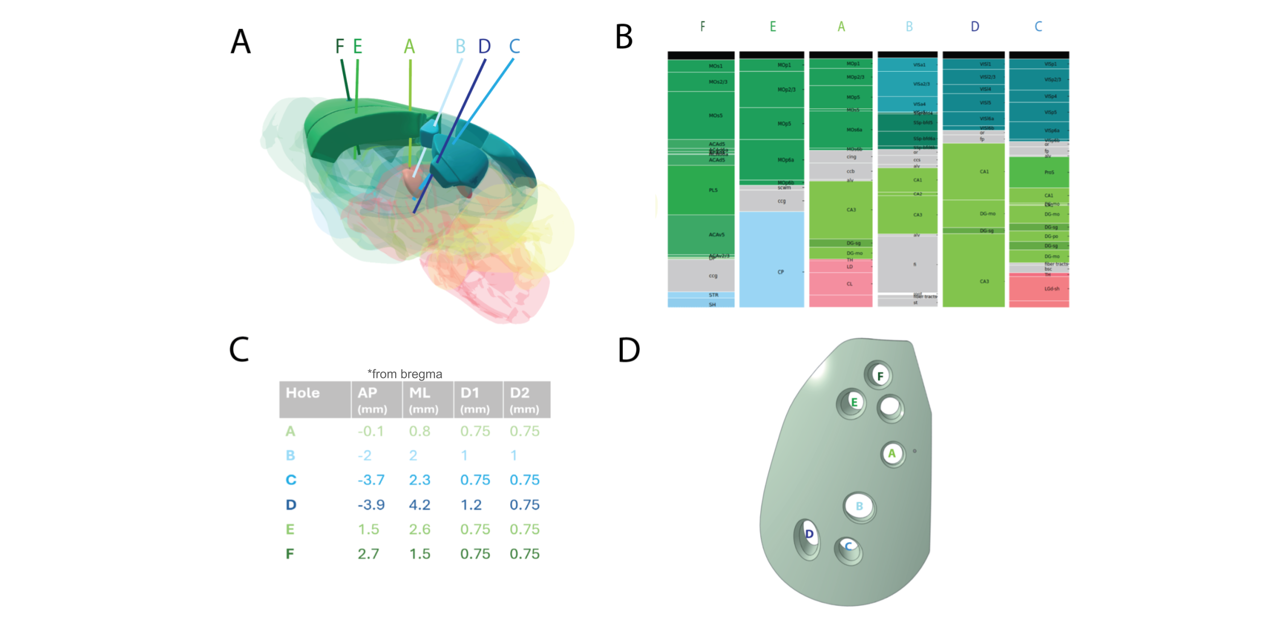
Supplementary Figure 1. Neuropixels implant geometry and planned probe trajectories. A, Six trajectories (A-F) through the Allen Mouse Brain Common Coordinate Framework. B, Atlas structures intersected by each trajectory. C, Anteroposterior and mediolateral coordinates relative to bregma with implant-hole diameters D1 and D2. D, Top view of the implant with labeled probe-access holes.
Supplementary Figure 2. Neuropixels unit yield across recording days. Individual lines show 60 sessions from 16 mice; the bold line shows the daily mean, and n is the number of sessions represented on each day. Units passed all three quality-control thresholds (ISI-violations ratio < 0.5, presence ratio > 0.8, and amplitude cutoff < 0.1). QC-passing units were divided by the number of recorded probes and normalized to each mouse’s day-1 value. Mean yield declined from 100% on day 1 to 80.9% on day 4. Values were derived from the public draft of Dandiset 001637 retrieved July 30, 2026.
Supplementary Figure 3. Recorded Neuropixels trajectories in the Allen Mouse
Brain Common Coordinate Framework (CCF) 2017. Line color denotes the nominal probe
port (A-F). A, an oblique projection shows the trajectories across the
depth-shaded whole-brain surface; B, a dorsal projection shows their
anteroposterior and mediolateral distribution. Both panels use a semi-transparent
brain surface, anatomical direction markers, and calibrated 2 mm scale bars;
the trajectories extend laterally toward the L direction marker, matching the
stereotaxic mediolateral convention. Electrode coordinates and area annotations
come from Dandiset 001637; the brain surface is a 100-micrometer mesh derived from the Allen CCF 2017
25-micrometer annotation volume. In total, 332 probe trajectories from 57 sessions and 16 mice
had finite CCF coordinates. Three of the 60 source sessions are excluded because
their NWB electrode tables lack x, y, and z coordinates.
Supplementary Figure 4. Synchronized eye tracking in selected Neuropixels (mouse 834687), mesoscope (mouse 839909), and SLAP2 (mouse 828409) sessions. Rows show raw pupil x position, y position, and area on a common time axis. The 16-second excerpts were selected to show a likely blink and a sustained change in pupil area; gray bands denote likely-blink samples. SLAP2 eye tracking is noisier than the other examples, consistent with illumination and whisker interference in the eye-camera view. Neuropixels and mesoscope videos are aligned using eye-camera exposure edges from the session sync files; SLAP2 uses packaged camera-frame indices and aligned Harp timestamps. All fit values and blink flags are from the corresponding public NWBs and are shown without display-time outlier interpolation.
Supplementary Figure 5. Peri-event pupil-area and running-speed responses across recording modalities, training cohorts, predictive-processing contexts, and mismatch events. A–B, Population mean event-minus-control pupil and running traces, aligned to display-synchronized stimulus onset and spanning −2 to 4 s. Pupil responses are percent changes from each trial’s median baseline; running responses are changes in forward speed (cm/s) from the mean baseline. The 45° and 90° orientation events are pooled for this summary. Shading denotes ±1 SEM across mice. C–D, Colored points show mouse effects, open circles show means, and vertical bars show 95% mouse-bootstrap intervals. Trials are averaged within session and repeated sessions within mouse; mice are the population sampling unit. The source snapshot includes 60 Neuropixels sessions from 16 mice, 86 mesoscope sessions from 10 mice, and 8 SLAP2 sessions from 3 mice. SLAP2 duration pupil responses are marked unavailable because each event or control retained fewer than three valid trials or less than 10% of presented trials after pupil quality control; running remains independently displayed where coverage is sufficient. Baseline definitions, control matching, signal processing, and exclusions are described in Methods. Data come from Dandisets 001637, 001768, and 001424.
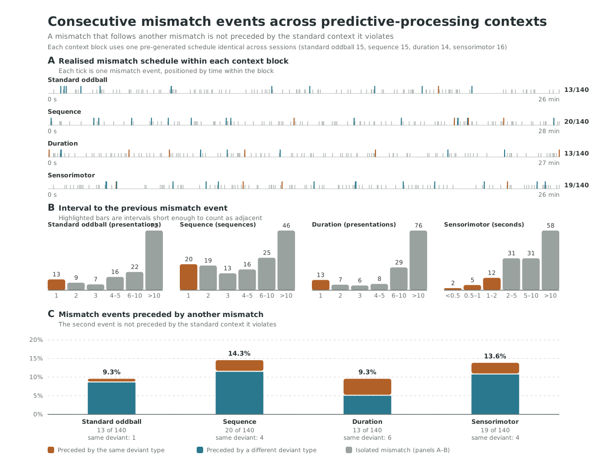
Supplementary Figure 6. Consecutive mismatch events across the four Neuropixels predictive-processing context blocks. A mismatch event that immediately follows another mismatch is not preceded by the standard context it violates, so its surprise is not comparable to that of an isolated mismatch. Adjacency is defined from each block’s structure: standard-oddball and duration blocks present one stimulus per stimulus-table row, so a deviant is adjacent when the preceding row is also a deviant; the sequence block presents five rows per sequence (four gratings then a grey inter-sequence interval) with the substitution always at the third element, so a substitution is adjacent when the previous sequence, five rows earlier, also substituted; the sensorimotor block embeds 350 ms mismatch events in a continuous 30 Hz phase-update stream, so adjacency is measured in elapsed time against the protocol’s intended 2 s minimum separation. Adjacency is evaluated only within a block. A, Each tick is one mismatch event positioned by its onset within the block; tall coloured ticks mark events preceded by another mismatch and short grey ticks mark isolated events. B, Interval to the previous mismatch event, binned in each context’s natural unit; highlighted bars are the intervals short enough to count as adjacent and sum to the counts in C. C, Percentage of mismatch events preceded by another mismatch, split by whether that preceding event was the same deviant type. Standard-oddball retains 13 of 140 adjacent events of which 1 repeats the deviant type, sequence 20 of 140 with 4 repeats, duration 13 of 140 with 6 repeats, and sensorimotor 19 of 140 with 4 repeats. Duration is the most affected because deviant delays repeat most often, and sensorimotor departs from its documented design: 19 pairs fall below the intended 2 s minimum, 7 below 1 s, and 2 below 0.5 s, with a floor of 0.450 s between onsets and 0.100 s between one event’s offset and the next event’s onset. Each context block uses one pre-generated stimulus schedule, verified identical across sessions by hashing the trial-type order, orientation, and delay columns, so these counts apply to every session and the extraction fails rather than averaging if a future release randomises the schedules. Values were measured from the stimulus interval tables of all 60 Neuropixels sessions in the public draft of Dandiset 001637: 15 standard-oddball, 15 sequence, 14 duration, and 16 sensorimotor blocks.
Supplementary Figure 7. Locomotion during the sensorimotor mismatch block across 39 Neuropixels and mesoscope sessions: 16 Neuropixels sessions from 16 mice and 23 mesoscope sessions from 10 mice. Sessions are grouped by modality and ordered by block mean forward speed. A, Block mean forward speed, with the 5 cm/s gate marked. B, Qualifying trials of 140 mismatch events at each reported threshold; darker cells indicate more qualifying trials. C, Qualifying trials for each of four mismatch event types, of 35 presentations each, colored by whether the type reaches the pre-registered eight-trial minimum. A trial qualifies only when mean forward speed reaches the threshold in both the 343 ms pre-event baseline and mismatch windows. Twenty-three of 39 sessions have a median speed of 0.00 cm/s. At 5 cm/s, 11 of 39 sessions meet the minimum in all four event types: 2 Neuropixels and 9 mesoscope sessions. Availability is assessed per event type; the matched open-loop control contains only 8 trials per type in every session. SLAP2 is excluded from this NWB-based analysis because its running measurements are packaged separately as Harp encoder files. Running processing, session-level coverage, and inclusion criteria are described in Methods. Values come from Dandisets 001637 and 001768.
Supplementary Text 1: Published oddball paradigms and sampling ranges
Supplementary Table 1 compares five published visual oddball paradigms with respect to stimulus design, timing, sample size, recording method, statistical test, habituation, and sampling.
Supplementary Table 1. Stimulus design, timing, sample size, recording method, statistical test, habituation, and sampling parameters for five published visual oddball paradigms. Each column describes one study; rows identify the compared parameters.
The paradigms span visuomotor decoupling and local or global deviations in visual sequences. Three studies used two-photon calcium imaging, one used local field potentials, and one used Neuropixels recordings.
Reported oddball probabilities ranged from 0.07 to 0.20, the reported number of oddball repeats required ranged from 10 to 144, and session durations ranged from 6 minutes to 2 hours. This comparison informed the mismatch repeat count and session duration used in the present dataset; differences in stimuli, response definitions, and significance tests should be considered when comparing responsive-neuron fractions across studies.
Glossary
Terms and abbreviations
Abbreviations indicate the relevant modality:
meso = mesoscopic 2-photon Ca2+-imaging
ephys = electro-physiology (neurophysiology) using Neuropixels probes
ophys = optical-physiology using any in vivo fluorescence imaging technique
slap2 = SLAP2 glutamate vesicle imaging
ROI (slap2): Region of interest: a localized candidate location of a synaptic spine.
(Single) Unit (ephys): A candidate for an isolated single neuron.
Receptive Field (meso/ephys/slap2): A region of sensory (here: visual) space where an isolated stimulus evokes a neuronal response (either increases or decreases neuronal activity).
Orientation Tuning (meso/ephys/slap2): The selective response of visual neurons to edges or bars at particular angles.
NWB: Neurodata Without Borders. Standardized file format specification that stores neuronal physiology data. Used to store data for all modalities in this work.
DANDI: The DANDI Archive (Distributed Archives for Neurophysiology Data Integration) is a public repository supported by the US BRAIN Initiative. It allows scientists to store, publish, and access cellular neurophysiology data, such as electrophysiology, optical physiology, and behavioral time-series.
- Aizenbud, I., Audette, N., Auksztulewicz, R., Basiński, K., Bastos, A. M., Berry, M., Canales-Johnson, A., Choi, H., Clopath, C., Cohen, U., Costa, R. P., De Filippo, R., Doronin, R., Durand, S., Errington, S. P., Gavornik, J. P., Gillon, C. J., Granier, A., Hamm, J. P., … Xiong, Y. S. (2026). Neural mechanisms of predictive processing: A collaborative community experiment through the OpenScope program. https://arxiv.org/abs/2504.09614v2
- de Vries, S. E. J., Lecoq, J. A., Buice, M. A., Groblewski, P. A., Ocker, G. K., Oliver, M., Feng, D., Cain, N., Ledochowitsch, P., Millman, D., Roll, K., Garrett, M., Keenan, T., Kuan, L., Mihalas, S., Olsen, S., Thompson, C., Wakeman, W., Waters, J., … Koch, C. (2020). A large-scale standardized physiological survey reveals functional organization of the mouse visual cortex. Nature Neuroscience, 23(1), 138–151. 10.1038/s41593-019-0550-9
- Groblewski, P. A., Sullivan, D., Lecoq, J., de Vries, S. E. J., Caldejon, S., L’Heureux, Q., Keenan, T., Roll, K., Slaughterback, C., Williford, A., & Farrell, C. (2020). A standardized head-fixation system for performing large-scale, in vivo physiological recordings in mice. Journal of Neuroscience Methods, 346, 108922. 10.1016/j.jneumeth.2020.108922
- Durand, S., Heller, G. R., Ramirez, T. K., Luviano, J. A., Williford, A., Sullivan, D. T., Cahoon, A. J., Farrell, C., Groblewski, P. A., Bennett, C., Siegle, J. H., & Olsen, S. R. (2023). Acute head-fixed recordings in awake mice with multiple Neuropixels probes. Nature Protocols, 18(2), 424–457. 10.1038/s41596-022-00768-6
- Bennett, C., Ouellette, B., Ramirez, T. K., Cahoon, A., Cabasco, H., Browning, Y., Lakunina, A., Lynch, G. F., McBride, E. G., Belski, H., Gillis, R., Grasso, C., Howard, R., Johnson, T., Loeffler, H., Smith, H., Sullivan, D., Williford, A., Caldejon, S., … Olsen, S. R. (2024). SHIELD: Skull-shaped hemispheric implants enabling large-scale electrophysiology datasets in the mouse brain. Neuron, 112(17), 2869-2885.e8. 10.1016/j.neuron.2024.06.015
- Siegle, J. H., Jia, X., Durand, S., Gale, S., Bennett, C., Graddis, N., Heller, G., Ramirez, T. K., Choi, H., Luviano, J. A., Groblewski, P. A., Ahmed, R., Arkhipov, A., Bernard, A., Billeh, Y. N., Brown, D., Buice, M. A., Cain, N., Caldejon, S., … Koch, C. (2021). Survey of spiking in the mouse visual system reveals functional hierarchy. Nature, 592(7852), 86–92. 10.1038/s41586-020-03171-x
- Harris, J. A., Hirokawa, K. E., Sorensen, S. A., Gu, H., Mills, M., Ng, L. L., Bohn, P., Mortrud, M., Ouellette, B., Kidney, J., Smith, K. A., Dang, C., Sunkin, S., Bernard, A., Oh, S. W., Madisen, L., & Zeng, H. (2014). Anatomical characterization of Cre driver mice for neural circuit mapping and manipulation. Frontiers in Neural Circuits, 8, 76. 10.3389/fncir.2014.00076
- Daigle, T. L., Madisen, L., Hage, T. A., Valley, M. T., Knoblich, U., Larsen, R. S., Takeno, M. M., Huang, L., Gu, H., Larsen, R., Mills, M., Bosma-Moody, A., Siverts, L. A., Walker, M., Graybuck, L. T., Yao, Z., Fong, O., Nguyen, T. N., Garren, E., … Zeng, H. (2018). A suite of transgenic driver and reporter mouse lines with enhanced brain-cell-type targeting and functionality. Cell, 174(2), 465-480.e22. 10.1016/j.cell.2018.06.035
- Zhang, Y., Rózsa, M., Liang, Y., Bushey, D., Wei, Z., Zheng, J., Reep, D., Broussard, G. J., Tsang, A., Tsegaye, G., Narayan, S., Obara, C. J., Lim, J.-X., Patel, R., Zhang, R., Ahrens, M. B., Turner, G. C., Wang, S. S.-H., Korff, W. L., … Looger, L. L. (2023). Fast and sensitive GCaMP calcium indicators for imaging neural populations. Nature, 615(7954), 884–891. 10.1038/s41586-023-05828-9
- Madisen, L., Mao, T., Koch, H., Zhuo, J., Berenyi, A., Fujisawa, S., Hsu, Y.-W. A., Garcia, A. J., Gu, X., Zanella, S., Kidney, J., Gu, H., Mao, Y., Hooks, B. M., Boyden, E. S., Buzsaki, G., Ramirez, J. M., Jones, A. R., Svoboda, K., … Zeng, H. (2012). A toolbox of Cre-dependent optogenetic transgenic mice for light-induced activation and silencing. Nature Neuroscience, 15(5), 793–802. 10.1038/nn.3078
- Taniguchi, H., He, M., Wu, P., Kim, S., Paik, R., Sugino, K., Kvitsani, D., Fu, Y., Lu, J., Lin, Y., Miyoshi, G., Shima, Y., Fishell, G., Nelson, S. B., & Huang, Z. J. (2011). A resource of Cre driver lines for genetic targeting of GABAergic neurons in cerebral cortex. Neuron, 71(6), 995–1013. 10.1016/j.neuron.2011.07.026
- Zhang, F., Wang, L.-P., Boyden, E. S., & Deisseroth, K. (2006). Channelrhodopsin-2 and optical control of excitable cells. Nature Methods, 3(10), 785–792. 10.1038/nmeth936
- Oommen, B. S., & Stahl, J. S. (2008). Eye orientation during static tilts and its relationship to spontaneous head pitch in the laboratory mouse. Brain Research, 1193, 57–66. 10.1016/j.brainres.2007.11.053
- Kalatsky, V. A., & Stryker, M. P. (2003). New paradigm for optical imaging: Temporally encoded maps of intrinsic signal. Neuron, 38(4), 529–545. 10.1016/S0896-6273(03)00286-1
- Marshel, J. H., Garrett, M. E., Nauhaus, I., & Callaway, E. M. (2011). Functional specialization of seven mouse visual cortical areas. Neuron, 72(6), 1040–1054. 10.1016/j.neuron.2011.12.004